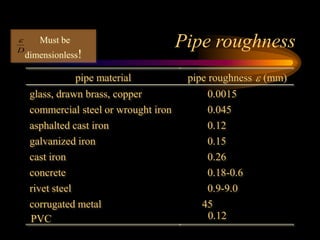
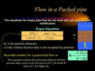
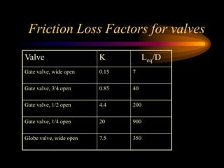
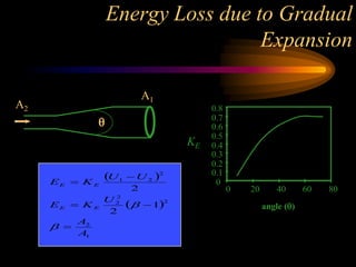
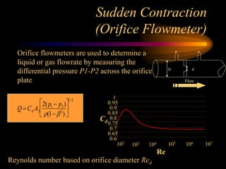
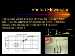
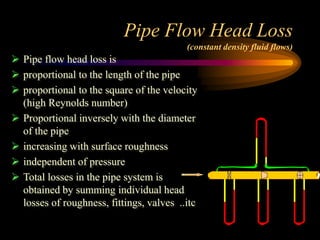
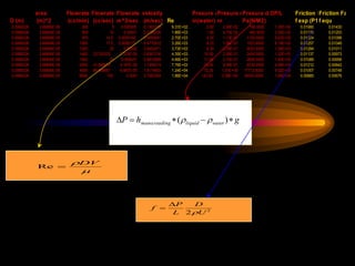
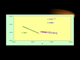
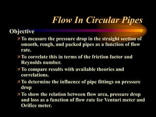
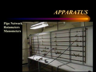
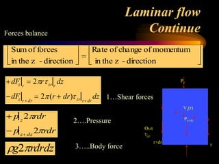
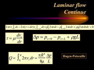
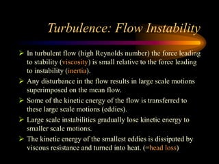
The document discusses flow in circular pipes. It outlines the objectives of measuring pressure drop in smooth, rough and packed pipes as a function of flow rate. It aims to correlate these measurements in terms of friction factor and Reynolds number. The apparatus used includes pipe networks, rotameters and manometers. Laminar and turbulent flow are examined theoretically using concepts like boundary layers, velocity profiles, friction factors and Reynolds number. Flow in valves, expansions, contractions and venturi/orifice meters is also analyzed. Head losses are shown to depend on length, velocity, diameter and roughness. Pipes are ubiquitous in nature, infrastructure and engineering systems.

1. Flow In Circular Pipes
Objective
 To measure the pressure drop in the straight section of
smooth, rough, and packed pipes as a function of flow
rate.
 To correlate this in terms of the friction factor and
Reynolds number.
 To compare results with available theories and
correlations.
 To determine the influence of pipe fittings on pressure
drop
 To show the relation between flow area, pressure drop
and loss as a function of flow rate for Venturi meter and
Orifice meter.

2. APPARATUS
Pipe Network
Rotameters
Manometers

3. Theoretical Discussion
Fluid flow in pipes is of considerable importance in process.
•Animals and Plants circulation systems.
•In our homes.
•City water.
•Irrigation system.
•Sewer water system
 Fluid could be a single phase: liquid or gases
Mixtures of gases, liquids and solids
 NonNewtonian fluids such as polymer melts, mayonnaise
 Newtonian fluids like in your experiment (water)

4. Theoretical Discussion
Laminar flow
To describe any of these flows, conservation of mass and
conservation of momentum equations are the most general forms
could be used to describe the dynamic system. Where the key
issue is the relation between flow rate and pressure drop.
If the flow fluid is:
a. Newtonian
b. Isothermal
c. Incompressible (dose not depend on the pressure)
d. Steady flow (independent on time).
e. Laminar flow (the velocity has only one single component)

5. Laminar flow
Navier-Stokes equations is govern the flow field (a set of equations
containing only velocity components and pressure) and can be solved
exactly to obtain the Hagen-Poiseuille relation
.
Vz(r)


In

Pz
r+dr r
Body force due to gravity
Flow If the principle of conservation
of momentum is applied to a
fixed volume element through
which fluid is flowing and on
which forces are acting, then
the forces must be balanced
(Newton second law)

Pz+dz
Pz+dz

6. Laminar flow
Continue
Forces balance
dFz r
 2rzr r
dz
dFz r  dr
 2(r  dr)zr r dr
dz 1…Shear forces
 p z
2rdr
 p z dz
2rdr
2….Pressure
g2rdrdz 3…..Body force
Sum of forces
in the z - direction






Rate of change of momentum
in the z - direction






Vz(r)


Pz
r+dr r
Pz+dz

7. Laminar flow
Continue
Momentum is
Mass*velocity (m*v)
Momentum per unit volume is
*vz
Rate of flow of momentum is
*vz*dQ
dQ=vz2πrdr
but
vz = constant at a fixed value of r
vz (v2rdr) z
 vz (v2rdr) z dz
 0
Laminar flow

8. Laminar flow
Continue
2rzr r
dz 2(r  dr)zr r dr
dzp z
2rdr p z dz
2rdr  g2rdrdz  0
  
dvz
dr
Q  2vz dr
0
R
 
R4
8
p
L
p  pz0  pzL  gL
Hagen-Poiseuille

9. Turbulent flow
When fluid flow at higher flowrates,
the streamlines are not steady and
straight and the flow is not laminar.
Generally, the flow field will vary in
both space and time with fluctuations
that comprise "turbulence
For this case almost all terms in the
Navier-Stokes equations are important
and there is no simple solution
P = P (D, , , L, U,)
uz
úz
Uz
average
ur
úr
Ur
average
p
P’
p
average
Time

10. Turbulent flow
All previous parameters involved three fundamental dimensions,
Mass, length, and time
From these parameters, three dimensionless groups can be build
P
U 2  f (Re,
L
D
)
Re 
UD


inertia
Viscous forces

11. Friction Factor for Laminar
Turbulent flows
From forces balance and the definition of Friction Factor
P  Ac   S  L
Ac
S
 rh 
1
4
D

P
2L
R
f 

1/2U2
For Laminar flow
(Hagen - Poiseuill eq)
Q 
r4
8
P
L
P
L

8U
R2
f 
PR
U
2
L
f 
P
L
R
U 2 
8
UR

16
Re
For Turbulent Flow f 
P
L
D
2U 2  0.079Re0.25
Ac: cross section area of the pip
S: Perimeter on which T acts (wetted
perimeter)
Rh hydraulic radius

12. Turbulence: Flow Instability
 In turbulent flow (high Reynolds number) the force leading
to stability (viscosity) is small relative to the force leading
to instability (inertia).
 Any disturbance in the flow results in large scale motions
superimposed on the mean flow.
 Some of the kinetic energy of the flow is transferred to
these large scale motions (eddies).
 Large scale instabilities gradually lose kinetic energy to
smaller scale motions.
 The kinetic energy of the smallest eddies is dissipated by
viscous resistance and turned into heat. (=head loss)

13. Velocity Distributions
Turbulence causes transfer of momentum
from center of pipe to fluid closer to the pipe
wall.
Mixing of fluid (transfer of momentum)
causes the central region of the pipe to have
relatively constant velocity (compared to
laminar flow)
Close to the pipe wall eddies are smaller (size
proportional to distance to the boundary)

14. Surface Roughness
Additional dimensionless group /D need
to be characterize
Thus more than one curve on friction factor-
Reynolds number plot
Fanning diagram or Moody diagram
Depending on the laminar region.
If, at the lowest Reynolds numbers, the laminar portion
corresponds to f =16/Re Fanning Chart
or f = 64/Re Moody chart

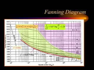
15. Friction Factor for Smooth, Transition,
and Rough Turbulent flow

1
f
 4.0 * log Re* f
 0.4
Smooth pipe, Re>3000

1
f
 4.0 * log
D

 2.28
Rough pipe, [ (D/)/(Re√ƒ) <0.01]
1
f
 4.0*log
D

 2.28 4.0*log 4.67
D/
Re f
1






Transition function
for both smooth and
rough pipe
f 
P
L
D
2U2

f  0.079Re0.25

16. Fanning Diagram
f =16/Re

f  0.079Re0.25

1
f
 4.0 * log
D

 2.28  4.0 * log 4.67
D/
Re f
1







1
f
 4.0 * log
D

 2.28

17. Pipe roughness
pipe material pipe roughness  (mm)
glass, drawn brass, copper 0.0015
commercial steel or wrought iron 0.045
asphalted cast iron 0.12
galvanized iron 0.15
cast iron 0.26
concrete 0.18-0.6
rivet steel 0.9-9.0
corrugated metal 45
PVC 0.12
Must be
dimensionless!

D

18. Flow in a Packed pipe
The equations for empty pipe flow do not work with out considerable
modification
Ergun Equation
75
.
1
)
1
(
150
)
1
(
2
3












p
o
o
p
D
U
U
L
PD
f
Reynolds number for a packed bed flow as Re 
UoDp
(1)
Dp is the particle diameter,
 is the volume fraction that is not occupied by particles
This equation contains the interesting behavior that the
pressure drop varies as the first power of Uo for small Re
and as Uo
2 for higher Re.
Flow
Dp
A

19. Energy Loss in Valves
 Function of valve type and valve position
 The complex flow path through valves can
result in high head loss (of course, one of
the purposes of a valve is to create head
loss when it is not fully open)
 Ev are the loss in terms of velocity heads
Ev  K
U2
2
hv 
p

 Kv
U2
2g
 2 f
Leq
D
U2
g

20. Friction Loss Factors for valves
Valve K Leq/D
Gate valve, wide open 0.15 7
Gate valve, 3/4 open 0.85 40
Gate valve, 1/2 open 4.4 200
Gate valve, 1/4 open 20 900
Globe valve, wide open 7.5 350

21. Energy Loss due to Gradual
Expansion
angle ()
0
0.1
0.2
0.3
0.4
0.5
0.6
0.7
0.8
0 20 40 60 80
KE

A2
A1
 
 
1
2
2
2
2
2
2
1
1
2
2
A
A
U
K
E
U
U
K
E
E
E
E
E








22. Sudden Contraction
(Orifice Flowmeter)
Orifice flowmeters are used to determine a
liquid or gas flowrate by measuring the
differential pressure P1-P2 across the orifice
plate
0.6
0.65
0.7
0.75
0.8
0.85
0.9
0.95
1
102 105 106 107
Re
Cd
Reynolds number based on orifice diameter Red
P1 P2
d
D
Flow
103 104
Q  Cd A2
2(p1  p2)
(12
)






1/2

23. Venturi Flowmeter
The classical Venturi tube (also known as the Herschel Venturi
tube) is used to determine flowrate through a pipe. Differential
pressure is the pressure difference between the pressure
measured at D and at d
D d Flow

24. Boundary layer buildup in a pipe
Pipe
Entrance
v v
v
Because of the share force near the pipe wall, a boundary layer
forms on the inside surface and occupies a large portion of the
flow area as the distance downstream from the pipe entrance
increase. At some value of this distance the boundary layer fills the
flow area. The velocity profile becomes independent of the axis in
the direction of flow, and the flow is said to be fully developed.

25. Pipe Flow Head Loss
(constant density fluid flows)
 Pipe flow head loss is
 proportional to the length of the pipe
 proportional to the square of the velocity
(high Reynolds number)
 Proportional inversely with the diameter
of the pipe
 increasing with surface roughness
 independent of pressure
 Total losses in the pipe system is
obtained by summing individual head
losses of roughness, fittings, valves ..itc

26. Pipe Flow Summary
The statement of conservation of mass, momentum and energy becomes
the Bernoulli equation for steady state constant density of flows.
 Dimensional analysis gives the relation between flow rate and pressure
drop.
Laminar flow losses and velocity distributions can be derived based on
momentum and mass conservation to obtain exact solution named of
Hagen - Poisuille
Turbulent flow losses and velocity distributions require experimental
results.
Experiments give the relationship between the fraction factor and the
Reynolds number.
 Head loss becomes minor when fluid flows at high flow rate (fraction
factor is constant at high Reynolds numbers).

27. Images - Laminar/Turbulent Flows
Laser - induced florescence image of an
incompressible turbulent boundary layer
Simulation of turbulent flow coming out of a
tailpipe
Laminar flow (Blood Flow)
Laminar flow
Turbulent flow
http://www.engineering.uiowa.edu/~cfd/gallery/lim-turb.html

28. Pipes are Everywhere!
Owner: City of
Hammond, IN
Project: Water Main
Relocation
Pipe Size: 54"

29. Pipes are Everywhere!
Drainage Pipes

31. Pipes are Everywhere!
Water Mains

33. area Flowrate Flowrate Flowrate velosity Presure drop
Presure drop
Presure drop
DP/L Friction Factor
Friction Facto
D (m) (m)^2 (cc/min) (cc/sec) m^3/sec (m/sec) Re in(water) m Pa(N/M2) f exp (P1)f equ
0.0068326 3.66806E-05 300 5 0.000005 0.1363118 9.31E+02 0.80 2.00E-02 196.0000 1.05E+02 0.01980 0.01430
0.0068326 3.66806E-05 600 10 0.00001 0.2726235 1.86E+03 1.90 4.75E-02 465.5000 2.50E+02 0.01176 0.01203
0.0068326 3.66806E-05 870 14.5 0.0000145 0.3953041 2.70E+03 4.50 1.13E-01 1102.5000 5.93E+02 0.01324 0.01096
0.0068326 3.66806E-05 1050 17.5 0.0000175 0.4770912 3.26E+03 6.22 1.56E-01 1523.9000 8.19E+02 0.01257 0.01046
0.0068326 3.66806E-05 1200 20 0.00002 0.5452471 3.73E+03 8.30 2.08E-01 2033.5000 1.09E+03 0.01284 0.01011
0.0068326 3.66806E-05 1400 23.333333 2.333E-05 0.6361216 4.35E+03 10.00 2.50E-01 2450.0000 1.32E+03 0.01137 0.00973
0.0068326 3.66806E-05 1500 25 0.000025 0.6815589 4.66E+03 11.00 2.75E-01 2695.0000 1.45E+03 0.01089 0.00956
0.0068326 3.66806E-05 2500 41.666667 4.167E-05 1.1359314 7.76E+03 34.00 8.50E-01 8330.0000 4.48E+03 0.01212 0.00842
0.0068326 3.66806E-05 4000 66.666667 6.667E-05 1.8174903 1.24E+04 72.30 1.81E+00 17713.5000 9.52E+03 0.01007 0.00748
0.0068326 3.66806E-05 6000 100 0.0001 2.7262354 1.86E+04 143.00 3.58E+00 35035.0000 1.88E+04 0.00885 0.00676

P  hmano.reading (liquid  water) g

f 
P
L
D
2U 2
Re 
DV


34. f = 0.079Re
-0.25
f = 0.0688Re
-
f = 16Re -1
1.00E-03
1.00E-02
1.00E-01
1.00E+00
1.00E+02 1.00E+03 1.00E+04 1.00E+05
Re
Friction
factor