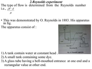
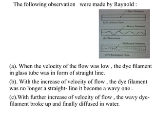
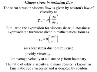
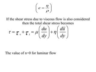
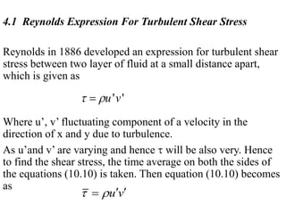
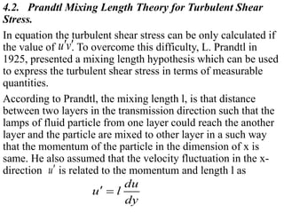
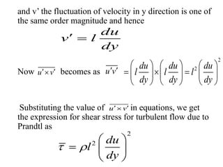
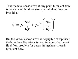
Mechanical Engineering Department
4th semester
Subject :- Fluid Mechanics
TOPIC :- TURBULENT FLOW
Prepared by :- Guided by :-
Sanjay Noelia (151120119022) prof. Dharmesh Jariwala
Prince Kumar (151120119031)
Abhishek Mishra (151120119001)
Niraj Pandey (151120119023)
• Introduction
• In the laminar flow the fluid particles moves along
straight parallel path in layer or lamina , such that the
path of individual fluid particles do no cross those of
neighboring particles .
• Laminar flow is possible only at low velocities and
when the fluid is highly viscous. But when the velocity
is increase or the fluid is less viscous , the fluid
particles do not move in straight path.
• The fluid particle moves in random manner resulting in
general mixing of the particles . This type of flow is
called turbulent flow.
A laminar flow changes to turbulent flow when :
1.Velocity is increase .
2.Diameter of pipe is increase .
3.Velocity of fluid is decreased .
O .Reynolds was the first to demonstrate that the
transition from laminar to turbulent depends not only
on the main velocity but not on the quantity .
• This quantity is a dimensionless quantity and is
called Reynolds number .
vD

eR
VD

In case of circular pipe if the flow is said
to be laminar and if then the floe is said to
be turbulent .
• If lies between 2000 to 4000 , the flow changes
from laminar to turbulent.i.e,
 Laminar when Re < 2000.
 Turbulent when Re > 4000.
 Transient when 2000 < Re < 4000.
2000eR 
4000eR 
eR
2.Reynolds experiment
The type of flow is determined from the Reynolds number
i.e.,
• This was demonstrated by O. Reynolds in 1883. His apparatus
in fig.
The apparatus consist of :
1) A tank contain water at constant head .
2) A small tank containing some dye.
3) A glass tube having a bell-mouthed entrance at one end and a
rectangular value at other end.
V d


The following observation were made by Raynold :
(a). When the velocity of the flow was low , the dye filament
in glass tube was in form of straight line.
(b). With the increase of velocity of flow , the dye filament
was no longer a straight- line it become a wavy one .
(c).With further increase of velocity of flow , the wavy dye-
filament broke up and finally diffused in water.
In case of laminar flow , the loss of pressure head was
found to be proportional to the velocity but in case of
turbulent flow , Reynolds observed that loss of head is
approximately proportional to the square of velocity .
More exactly the loss of head , where
varies from 1.75 to 2.0 .
n
fh v n
 3 . Frictional loss in pipe flow
When a liquid is flowing through a pipe ,the velocity of the liquid
layer adjacent to the pipe wall is zero the velocity of liquid is goes
to increasing from the wall and thus velocity gradient and hence
shear stress are produce in the whole liquid due to viscosity. This
viscous action causes loss of energy which is usually known as
frictional loss.
On the basis of his experiments, William Froude gave the laws of
fluid fraction for turbulent flow
The frictional resistance for the turbulent flow is :
(1) Proportional to V n ,where n varies from 1.5 to 2.0,
(2) Proportional to the density of fluid,
(3) Proportional to the area of surface in contact,
(4) Independent of pressure
(5) Dependent on the nature of the surface in contact.
3.1 Expression for loss of head due to friction in pipes.
Consider a uniform horizontal pipe, having steady flow as
shown in fig. 10.3. Let 1-1 and 2-2 are two section of pipe.
Le P1 = pressure intensity at section 1-1,
V1 = Velocity of flow at section 1-1,
L = Length of pipe between section 1-1 and 2-2,
d = diameter of pipe
= frictional resistance per unit wetted area per unit velocity
h f = loss of head due to friction,
P2, V2 = are value of pressure intensity and velocity at
section 2-2,
f 
Applying Bernoulli’s equation between section 1-1 and 2-2
Total heat at 1-1 = Total heat 2-2 + loss of head due to friction
between 1-1 and 2-2
Z1 = Z2 as pipe is horizontal
V1 = V2 as dia. Of pipe is same at 1-1 and 2-2
but is the head lost due to friction and hence intensity of
pressure will be reduced in the direction of flow by frictional
resistance.
22
1 2 2
1 2
2 2
f
p p vv
z z h
g g g g 
     
1 2
f
p p
h
g g 
 
fh
Now frictional resistance = frictional per unit wetted area per
unit velocity wetted area velocity2
The force acting on the fluid between section 1-1 and 2-2 are:
1. Pressure force at section 1-1 = P A
2. Pressure of at section 2-2 = P2 A
3. Frictional force f1 as shown in fig.
Resolving all forces in horizontal direction ,we have
 
2
1 'F f dL V  


1 2 1 0p A p A F  
2
f P L V   
But from equation (1)
Equating the value of (p1-p2) we get
In equation (3)
  2
1 2 1
2
1 2
'
'
P P A F f P L V
f P L V
P P
A
     
  
 
1 2 fp p gh 
2
2
'
'
f
f
f p l v
gh
A
f P
h L V
g A


  

   
2
4
4
P Wettedperimeter d
A Area dd


  
Putting where f is known is co-efficient of
friction.
Equation (4) becomes as
Equations (4) is known as Darcy- Weisbach equation.
This equation commonly used for finding loss of head
due to friction in pipes.
Sometimes equation written as
Then f is known as friction factor.
2
2' 4 ' 4
f
f f LV
h L V
g d g d 
     
'
,
2
f f


2 2
4. 4 . .
.
2 2
f
f LV f LV
h
g d d g
 

2
. .
2
f
f L V
h
d g


3.2 Expression for co-efficient in terms of shear stress.
The equation gives forces acting between in section 1-1 and
2-2 in horizontal direction as
Force due to shear stress
shear stress*surface area
Cancelling πd from both sides we have
Equation can be written as
11 2
0A Ap p F  
21 1
( )App F  
  2
1 2
4
p p d t d L

    
 1 2
4
d
p p L  
 1 2 4
L
p p
d
  
2
1 2 4 . .
2f
p p f LV
g
g dh 
 
   
 
 
2
1 2
4. . .
2
f LV
p p g
d g

 
   
 
Equating the value of (P1-P2) in equation
2
4. . .
4
2
L f LV
g
d d g
 
 
   
 
2 2
2 2
fV g fV
g
g g

 

  
2
2
V
f


 
  
 
2
2
f
v



4.Shear stress in turbulent flow
The shear stress in viscous flow is given by newton's law of
viscosity as
Similar to the expression for viscous shear ,J. Bossiness
expressed the turbulent shear in mathematical form as
τt= shear stress due to turbulence
ῃ=eddy viscosity
ū= average velocity at a distance y from boundary
The ratio of eddy viscosity and mass density is known as
kinematic eddy viscosity and is denoted by epsilon
v
du
dy

 
  
 
t
du
dy

 
  
 
If the shear stress due to viscous flow is also considered
then the total shear stress becomes
The value of n=0 for laminar flow



 
 
 
v t
du du
dy dy
   
   
      
   
4.1 Reynolds Expression For Turbulent Shear Stress
Reynolds in 1886 developed an expression for turbulent shear
stress between two layer of fluid at a small distance apart,
which is given as
Where u’, v’ fluctuating component of a velocity in the
direction of x and y due to turbulence.
As u’and v’ are varying and hence  will be also very. Hence
to find the shear stress, the time average on both the sides of
the equations (10.10) is taken. Then equation (10.10) becomes
as
' 'u v 
u v   
4.2. Prandtl Mixing Length Theory for Turbulent Shear
Stress.
In equation the turbulent shear stress can be only calculated if
the value of . To overcome this difficulty, L. Prandtl in
1925, presented a mixing length hypothesis which can be used
to express the turbulent shear stress in terms of measurable
quantities.
According to Prandtl, the mixing length l, is that distance
between two layers in the transmission direction such that the
lamps of fluid particle from one layer could reach the another
layer and the particle are mixed to other layer in a such way
that the momentum of the particle in the dimension of x is
same. He also assumed that the velocity fluctuation in the x-
direction is related to the momentum and length l as
u v 
u
du
u l
dy
 
and v’ the fluctuation of velocity in y direction is one of
the same order magnitude and hence
Now becomes as
Substituting the value of in equations, we get
the expression for shear stress for turbulent flow due to
Prandtl as
du
v l
dy
 
u v  u v 
2
2du du du
l l l
dy dy dy
     
       
     
u v 
2
2 du
l
dy
 
 
  
 
Thus the total shear stress at any point turbulent flow
is the same of the shear stress in turbulent flow due to
Prandtl as
But the viscous shear stress is negligible except near
the boundary. Equations is used in most of turbulent
fluid flow problem for determining shear stress in
turbulent flow.
2
2du du
l
dy dy
  
 
   
 
THANK YOU

Fm final ppt

  • 1.
    Mechanical Engineering Department 4thsemester Subject :- Fluid Mechanics TOPIC :- TURBULENT FLOW Prepared by :- Guided by :- Sanjay Noelia (151120119022) prof. Dharmesh Jariwala Prince Kumar (151120119031) Abhishek Mishra (151120119001) Niraj Pandey (151120119023)
  • 2.
    • Introduction • Inthe laminar flow the fluid particles moves along straight parallel path in layer or lamina , such that the path of individual fluid particles do no cross those of neighboring particles . • Laminar flow is possible only at low velocities and when the fluid is highly viscous. But when the velocity is increase or the fluid is less viscous , the fluid particles do not move in straight path. • The fluid particle moves in random manner resulting in general mixing of the particles . This type of flow is called turbulent flow.
  • 3.
    • Introduction • Inthe laminar flow the fluid particles moves along straight parallel path in layer or lamina , such that the path of individual fluid particles do no cross those of neighboring particles . • Laminar flow is possible only at low velocities and when the fluid is highly viscous. But when the velocity is increase or the fluid is less viscous , the fluid particles do not move in straight path. • The fluid particle moves in random manner resulting in general mixing of the particles . This type of flow is called turbulent flow.
  • 4.
    A laminar flowchanges to turbulent flow when : 1.Velocity is increase . 2.Diameter of pipe is increase . 3.Velocity of fluid is decreased . O .Reynolds was the first to demonstrate that the transition from laminar to turbulent depends not only on the main velocity but not on the quantity . • This quantity is a dimensionless quantity and is called Reynolds number . vD  eR VD 
  • 5.
    In case ofcircular pipe if the flow is said to be laminar and if then the floe is said to be turbulent . • If lies between 2000 to 4000 , the flow changes from laminar to turbulent.i.e,  Laminar when Re < 2000.  Turbulent when Re > 4000.  Transient when 2000 < Re < 4000. 2000eR  4000eR  eR
  • 6.
    2.Reynolds experiment The typeof flow is determined from the Reynolds number i.e., • This was demonstrated by O. Reynolds in 1883. His apparatus in fig. The apparatus consist of : 1) A tank contain water at constant head . 2) A small tank containing some dye. 3) A glass tube having a bell-mouthed entrance at one end and a rectangular value at other end. V d  
  • 7.
    The following observationwere made by Raynold : (a). When the velocity of the flow was low , the dye filament in glass tube was in form of straight line. (b). With the increase of velocity of flow , the dye filament was no longer a straight- line it become a wavy one . (c).With further increase of velocity of flow , the wavy dye- filament broke up and finally diffused in water.
  • 8.
    In case oflaminar flow , the loss of pressure head was found to be proportional to the velocity but in case of turbulent flow , Reynolds observed that loss of head is approximately proportional to the square of velocity . More exactly the loss of head , where varies from 1.75 to 2.0 . n fh v n
  • 9.
     3 .Frictional loss in pipe flow When a liquid is flowing through a pipe ,the velocity of the liquid layer adjacent to the pipe wall is zero the velocity of liquid is goes to increasing from the wall and thus velocity gradient and hence shear stress are produce in the whole liquid due to viscosity. This viscous action causes loss of energy which is usually known as frictional loss. On the basis of his experiments, William Froude gave the laws of fluid fraction for turbulent flow The frictional resistance for the turbulent flow is : (1) Proportional to V n ,where n varies from 1.5 to 2.0, (2) Proportional to the density of fluid, (3) Proportional to the area of surface in contact, (4) Independent of pressure (5) Dependent on the nature of the surface in contact.
  • 10.
    3.1 Expression forloss of head due to friction in pipes. Consider a uniform horizontal pipe, having steady flow as shown in fig. 10.3. Let 1-1 and 2-2 are two section of pipe. Le P1 = pressure intensity at section 1-1, V1 = Velocity of flow at section 1-1, L = Length of pipe between section 1-1 and 2-2, d = diameter of pipe = frictional resistance per unit wetted area per unit velocity h f = loss of head due to friction, P2, V2 = are value of pressure intensity and velocity at section 2-2, f 
  • 11.
    Applying Bernoulli’s equationbetween section 1-1 and 2-2 Total heat at 1-1 = Total heat 2-2 + loss of head due to friction between 1-1 and 2-2 Z1 = Z2 as pipe is horizontal V1 = V2 as dia. Of pipe is same at 1-1 and 2-2 but is the head lost due to friction and hence intensity of pressure will be reduced in the direction of flow by frictional resistance. 22 1 2 2 1 2 2 2 f p p vv z z h g g g g        1 2 f p p h g g    fh
  • 12.
    Now frictional resistance= frictional per unit wetted area per unit velocity wetted area velocity2 The force acting on the fluid between section 1-1 and 2-2 are: 1. Pressure force at section 1-1 = P A 2. Pressure of at section 2-2 = P2 A 3. Frictional force f1 as shown in fig. Resolving all forces in horizontal direction ,we have   2 1 'F f dL V     1 2 1 0p A p A F   2 f P L V   
  • 13.
    But from equation(1) Equating the value of (p1-p2) we get In equation (3)   2 1 2 1 2 1 2 ' ' P P A F f P L V f P L V P P A            1 2 fp p gh  2 2 ' ' f f f p l v gh A f P h L V g A           2 4 4 P Wettedperimeter d A Area dd     
  • 14.
    Putting where fis known is co-efficient of friction. Equation (4) becomes as Equations (4) is known as Darcy- Weisbach equation. This equation commonly used for finding loss of head due to friction in pipes. Sometimes equation written as Then f is known as friction factor. 2 2' 4 ' 4 f f f LV h L V g d g d        ' , 2 f f   2 2 4. 4 . . . 2 2 f f LV f LV h g d d g    2 . . 2 f f L V h d g  
  • 15.
    3.2 Expression forco-efficient in terms of shear stress. The equation gives forces acting between in section 1-1 and 2-2 in horizontal direction as Force due to shear stress shear stress*surface area Cancelling πd from both sides we have Equation can be written as 11 2 0A Ap p F   21 1 ( )App F     2 1 2 4 p p d t d L        1 2 4 d p p L    1 2 4 L p p d    2 1 2 4 . . 2f p p f LV g g dh         
  • 16.
      2 1 2 4.. . 2 f LV p p g d g          Equating the value of (P1-P2) in equation 2 4. . . 4 2 L f LV g d d g           2 2 2 2 fV g fV g g g        2 2 V f          2 2 f v   
  • 17.
    4.Shear stress inturbulent flow The shear stress in viscous flow is given by newton's law of viscosity as Similar to the expression for viscous shear ,J. Bossiness expressed the turbulent shear in mathematical form as τt= shear stress due to turbulence ῃ=eddy viscosity ū= average velocity at a distance y from boundary The ratio of eddy viscosity and mass density is known as kinematic eddy viscosity and is denoted by epsilon v du dy         t du dy        
  • 18.
    If the shearstress due to viscous flow is also considered then the total shear stress becomes The value of n=0 for laminar flow          v t du du dy dy                   
  • 19.
    4.1 Reynolds ExpressionFor Turbulent Shear Stress Reynolds in 1886 developed an expression for turbulent shear stress between two layer of fluid at a small distance apart, which is given as Where u’, v’ fluctuating component of a velocity in the direction of x and y due to turbulence. As u’and v’ are varying and hence  will be also very. Hence to find the shear stress, the time average on both the sides of the equations (10.10) is taken. Then equation (10.10) becomes as ' 'u v  u v   
  • 20.
    4.2. Prandtl MixingLength Theory for Turbulent Shear Stress. In equation the turbulent shear stress can be only calculated if the value of . To overcome this difficulty, L. Prandtl in 1925, presented a mixing length hypothesis which can be used to express the turbulent shear stress in terms of measurable quantities. According to Prandtl, the mixing length l, is that distance between two layers in the transmission direction such that the lamps of fluid particle from one layer could reach the another layer and the particle are mixed to other layer in a such way that the momentum of the particle in the dimension of x is same. He also assumed that the velocity fluctuation in the x- direction is related to the momentum and length l as u v  u du u l dy  
  • 21.
    and v’ thefluctuation of velocity in y direction is one of the same order magnitude and hence Now becomes as Substituting the value of in equations, we get the expression for shear stress for turbulent flow due to Prandtl as du v l dy   u v  u v  2 2du du du l l l dy dy dy                     u v  2 2 du l dy         
  • 22.
    Thus the totalshear stress at any point turbulent flow is the same of the shear stress in turbulent flow due to Prandtl as But the viscous shear stress is negligible except near the boundary. Equations is used in most of turbulent fluid flow problem for determining shear stress in turbulent flow. 2 2du du l dy dy           
  • 23.