11

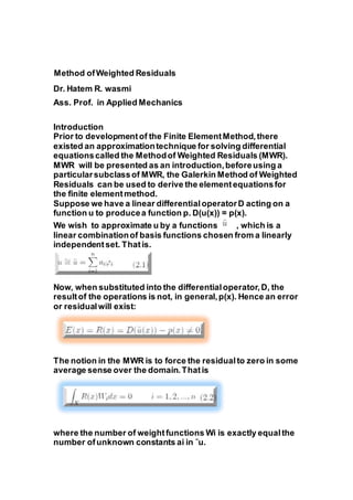
1. Method ofWeighted Residuals
Dr. Hatem R. wasmi
Ass. Prof. in Applied Mechanics
Introduction
Prior to developmentof the Finite ElementMethod,there
existed an approximationtechnique for solving differential
equationscalled the Methodof Weighted Residuals (MWR).
MWR will be presented as an introduction,beforeusing a
particularsubclassof MWR, the Galerkin Method of Weighted
Residuals can be used to derive the elementequationsfor
the finite elementmethod.
Suppose we have a linear differentialoperatorD acting on a
function u to producea function p. D(u(x)) = p(x).
We wish to approximate u by a functions , which is a
linear combinationof basis functions chosen from a linearly
independentset. Thatis.
Now, when substituted into the differentialoperator,D, the
resultof the operations is not, in general,p(x). Hence an error
or residualwill exist:
The notion in the MWR is to force the residualto zero in some
average sense over the domain.Thatis
where the number of weightfunctions Wi is exactly equalthe
number ofunknown constants ai in ˜u.

2. There are (at least) five MWR sub-methods,
accordingto the choices for the Wi’.
• Thesefive methods are:
1. collocation method.
2. Sub-domain method.
3. LeastSquares method.
4. Galerkin method.
5. Methodof moments.
2.1 Collocation Method
In this method,the weighting functions are taken from the
family of Dirac δ functions in the domain.
2.2 Sub-domain Method
This method doesn’tuse weighting factors explicity,so it is
not, strictly speaking,a member ofthe Weighted Residuals
family.
However,it can be considered a modification of the
collocation method.
The idea is to force the weighted residualto zero not just at
fixed points in the domain,but over varioussubsectionsof
the domain.
To accomplish this,the weight functions are setto unity, and
the integralover the entire domain is broken into a numberof
subdomainssufficientto evaluate all unknownparameters.

3. 2.3 LeastSquares Method
• If the continuous summationof all the squaredresiduals
is minimized,the rationale behind the name can be seen.
In other words,a minimum of
In order to achievea minimum of this scalar function,the
derivatives of S with respectto all the unknown parameters
must be zero.Thatis,
Comparing with 2.2, the weightfunctions are seen to be
however,the “2” can be dropped to get the weightfunction
for least square is
2.4 Galerkin Method
This method may be viewed as a modification of the Least
Squares Method.Rather than using the derivativeof the
residualwith respectto the unknownai, the derivative ofthe
approximating function is used.

4. Thatis, if the function is approximated as in 2.1, then the
weightfunctions are
Note that these are then identicalto the originalbasis
functions appearing in 2.1
2.5 Method of Moments
In this method,the weight functions are chosen from the
family of polynomials.Thatis
In the eventthat the basis functions for the approximation
(the ϕi’s) were chosen as polynomial,then the method of
moments may be identical to the Galerkin method.
Example (1)
As an example,considerthe solution of the following
mathematicalproblem.Find u(x) that satisfies

5. Solution
Note that for this problemthe differentialoperatorD(u(x)) and
p(x) are
For reference,the exactsolution can be found and is, in
generalform,
and for the given boundary conditions the constants can be
evaluated
So the exactsolution is
Let’s solve by the Methodof Weighted Residuals using a
polynomialfunction as a basis.Thatis, let the approximating
function be

6. and the approximatingpolynomialwhich also satisfies the
boundaryconditions is then
To find the residualR(x), we need the secondderivative of this
function,
So the residualis
Collocation Method
The residualis forced to zero at a number ofdiscretepoints.
Since there is only one unknown (a2),only one
collocation pointis needed.
We choose(arbitrarily,but from symmetryconsiderations)the
collocation pointx = 0.5.
Thus,the equation needed to evaluate the unknown a2 is

7. R(0.5) = −0.5 + a2(0.25 − .5 + 2) = 0
So
a2 = +0.5/1.75 = 2/7 = 0.285714
Subdomain Method
Since we have one unknownconstant,we choosea single
“sub-domain” which coversthe entire range of x. Therefore,
the relation to evaluate the constanta2 is
Least-Squares Method
The weightfunction W1 is just the derivative ofR(x) with
respectto the unknown a2:
So the weighted residual statementbecomes

8. Galerkin Method
In the Galerkin Method,the weightfunction W1 is the
derivativeof the approximatingfunction with respectto
the unknowncoefficienta2:
Method ofMoments
Since we have only one unknown coefficient,the weight function
W1(x) is simply
RMS Errors
A reasonable scalarindex for the closeness of two functions
is the L2 norm,or Euclidian norm.This measure is often
called the root-mean squared (RMS)error in engineering.The
RMS errorcan be defined as

9. The RMS errorsfor the differentapproximations are shownin
the last line of Table2.1. Note that these RMS errors are all
similar in magnitude,and that the Galerkin method has a
slightly lower RMS error than the others.
Comparison
A table of the tabulated valuesresultingfrom the different
approximationsis shown in Table 2.1 below