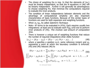
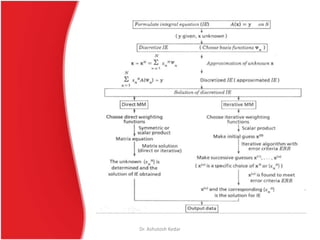
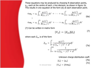
The document discusses the method of moments (MoM), a computational technique in electromagnetic analysis, detailing its historical development and theoretical foundations. It outlines the procedural steps for transforming linear functional equations into matrix equations and explains the application of MoM to wire antennas and other electromagnetic structures. The content includes various mathematical formulations and methods for solving electromagnetic problems, emphasizing the choice of basis and testing functions for accuracy.


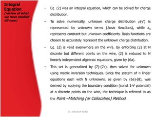
![Consider the deterministic equation
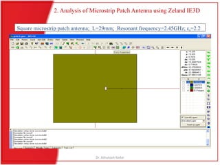
Lf=g (1)
Let f is represented by a set of functions {f1,f2,f3,….} in the domain of L as a linear
combination
(2)
Where aj are scalars to be determined; fj are called expansion functions or basis
functions.
For approximate solutions (2) is a finite summation; for exact solution it is usually an
infinite summation. Substitute (2) into (1) and using linearity of L, we have
(3)
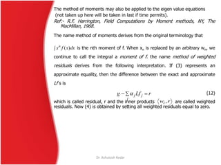
where the equality is usually approximate. Now defining a set of testing functions or
weighting functions {w1, w2, w3,….}in the range of L.
Take the inner product (usually an integration) of (3) with each wi, and use the linearity
of the inner product to obtain
(4)
j
jj ff
gLf jj
gwLfw ijij ,,
i=1,2,3,….This set of equations can be written in matrix form as
(5)
where [l] is the matrix
(6)
gl
ii Lfwl ,
Dr. Ashutosh Kedar
Method of
Moments](https://image.slidesharecdn.com/momslideshow-101103224202-phpapp01/85/Mom-slideshow-9-320.jpg)
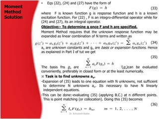
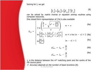
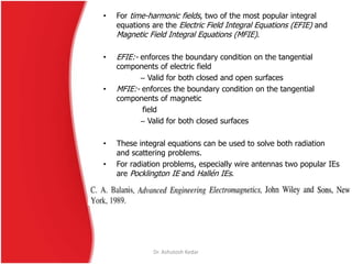
![and and g are column vectors
(7)
(8)
and if [l] is singular, its inverse exists, and i given as
(9)
The solution of f is then given by (2). For concise notation, define the row vector
of functions
(10)
Write (2) as and substitute from (9). The results is
(11)
This solution may be either approximate or exact, depending upon the choice
of expansion functions and testing functions.
gwg i
j
,
gl 1
jff
~
ff
~
1~
lff
Dr. Ashutosh Kedar](https://image.slidesharecdn.com/momslideshow-101103224202-phpapp01/85/Mom-slideshow-10-320.jpg)
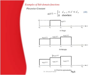
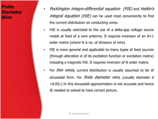
![1. Eigenfunction method
The eigenfunction method is the special case for which the expansion
functions are taken to be eigen functions of L, and the testing functions,
eigen functions of the adjoint operator, La. Its difficult to find these eigen
functions, but once known the solution of Lf=g is simple.
In this case, the matrix [l] of (5) is diagonal, with elements equal to the
eigen values, i , when the eigen functions are normalized or
bioorthogonalized. The inverse [l]-1 then has diagonal elements and the
moment solution (11) reduces to eigenfunctions solutions.
2. Galerkin’s method
When the domains of L and La are the same, we can chose wi = fi, and
the specialization is known as Galerkin’s method. When L is self-adjoint,
this has advantage of making [l] a symmetric matrix. Since the solution of
symmetric matrices is easy compared to non-symmetric, particularly for
eigen value problems, this can be a theoretical advantage. However, for
computations, the evaluation of the elements of [l] may be difficult when
Galerkin’s method is used and this outweighs the advantage of keeping [l]
symmetric.
1
i
Dr. Ashutosh Kedar
Specializations
of the Method
of Moments](https://image.slidesharecdn.com/momslideshow-101103224202-phpapp01/85/Mom-slideshow-12-320.jpg)

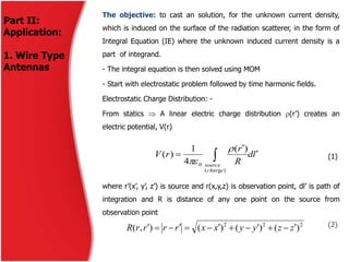
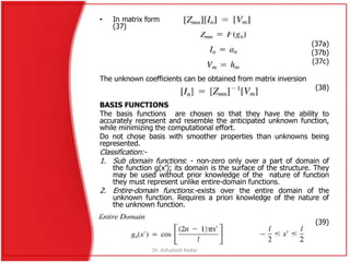
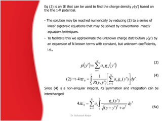
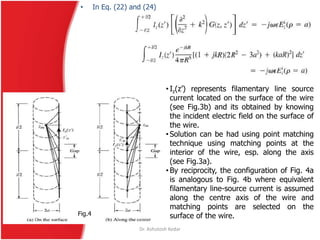
![(1) may be used to calculate the potential that are due to any known line
charge density.
difficult for complex geometries, unknown line charge density-use of IE-
MOM technique for solving.
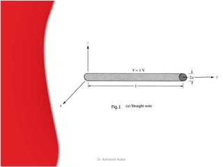
(A). Finite Straight Wire
The wire is of length l, and cross-sectional area a and is assumed to have
normalized constant electric potential of 1V. (1) is valid everywhere
including surface of the wire. Thus choosing the observation along the
wire axis (x=z=0) and representing the charge density of the wire as
(2)
where
(2a)
The observation point is chosen along the wire axis and the charge
density is expressed along the surface of wire so as to avoid R(y, y’)=0,
which would introduce singularity in integrand of (2).
lyyd
yyR
yl
0;
),(
)(
4
1
1
0
0
22
222
0
)(
])[()(),(),(
ayy
zxyyrrRyyR zx
Dr. Ashutosh Kedar](https://image.slidesharecdn.com/momslideshow-101103224202-phpapp01/85/Mom-slideshow-15-320.jpg)


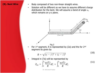
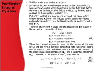


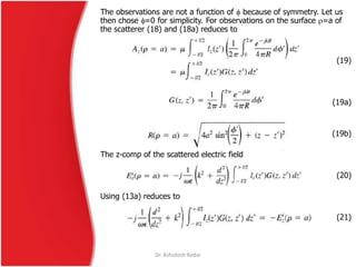

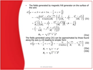
![• Referring to Fig. 3a, let us assume that the length of the cylinder is
much larger than its radius (l >> a) and its radius , a<<, so that
effects of the end faces of the cylinder can be neglected. Therefore
the boundary conditions for a wire with infinite conductivity are those
of vanishing total tangential E fields on the surface of the cylinder and
vanishing currents at the ends of the cylinder [ Iz (z’=±l /2)=0].
• Since only an electric current density flows on the cylinder and it is
directed along the z-axis (J=âz Jz), then A=âz Az (z’), which for smaller
radii is assumed to be a function of z’.
(25)
• Applying the boundary condition (vanishing tang. Elect. field)
(25a)
• Solution for (25a) assuming symmetry of current distribution
(26)
where B1 and C1 are constants. Using vector potential defn. (Balanis), we
obtain
(27)
C1=Vi/2 (if Vi is the input voltage) and B1 is obtained from B.C. that
current vanishes at the ends. (27) is Hallén’s Integral equation for
perfectly conducting wire.
Hallén’s
Integral
Equation
Dr. Ashutosh Kedar](https://image.slidesharecdn.com/momslideshow-101103224202-phpapp01/85/Mom-slideshow-32-320.jpg)