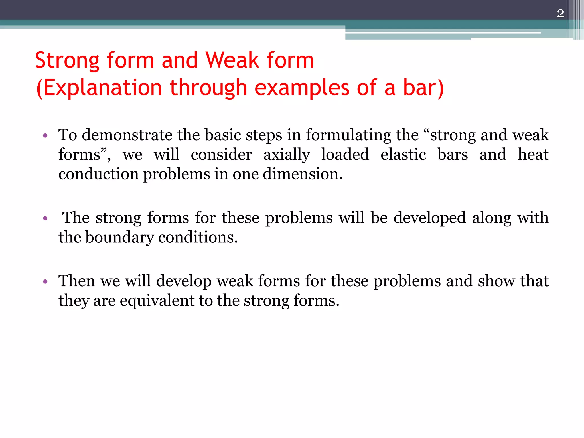
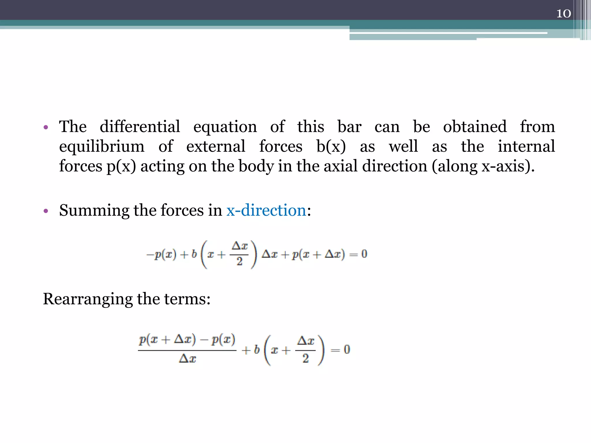
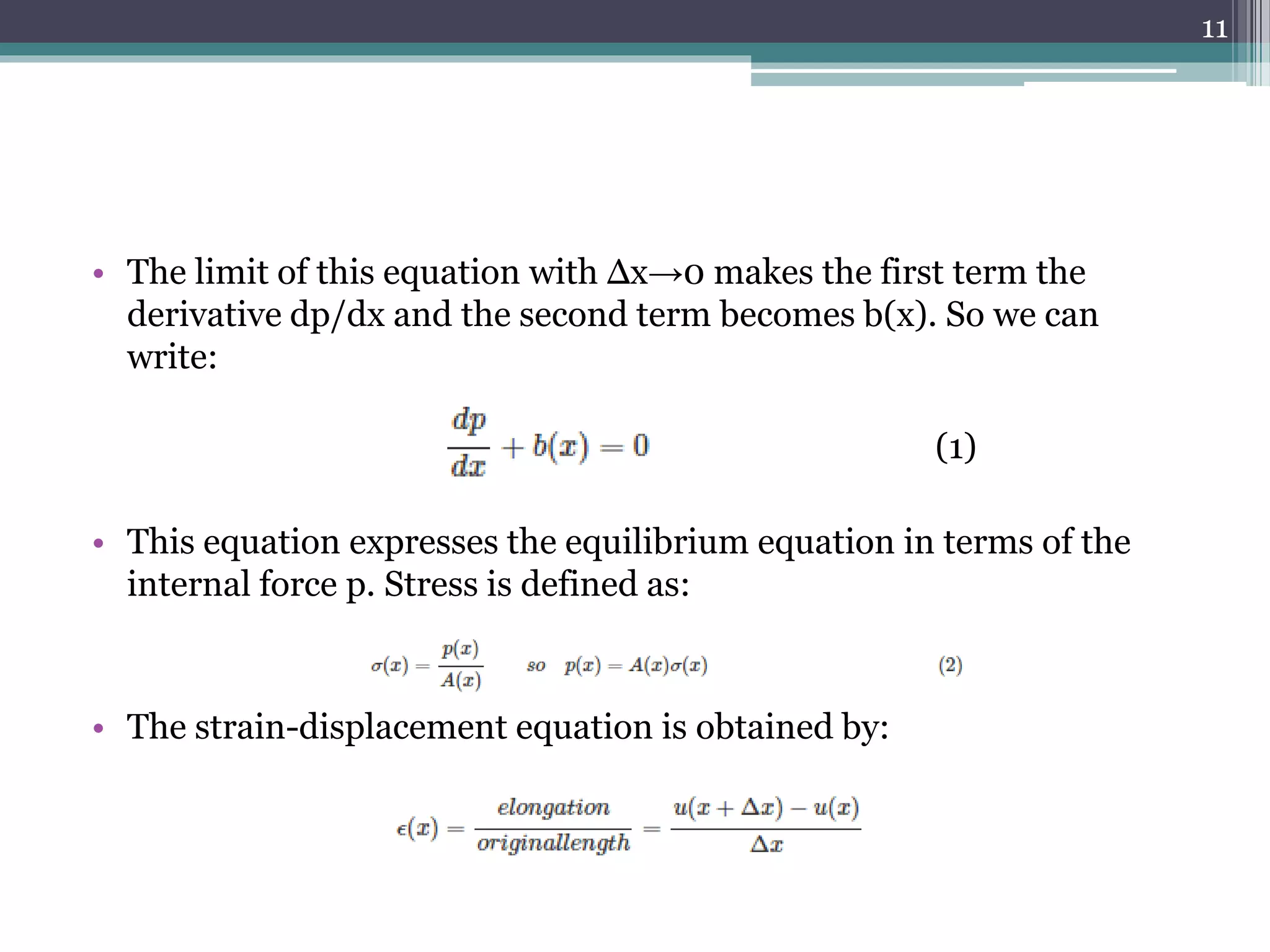
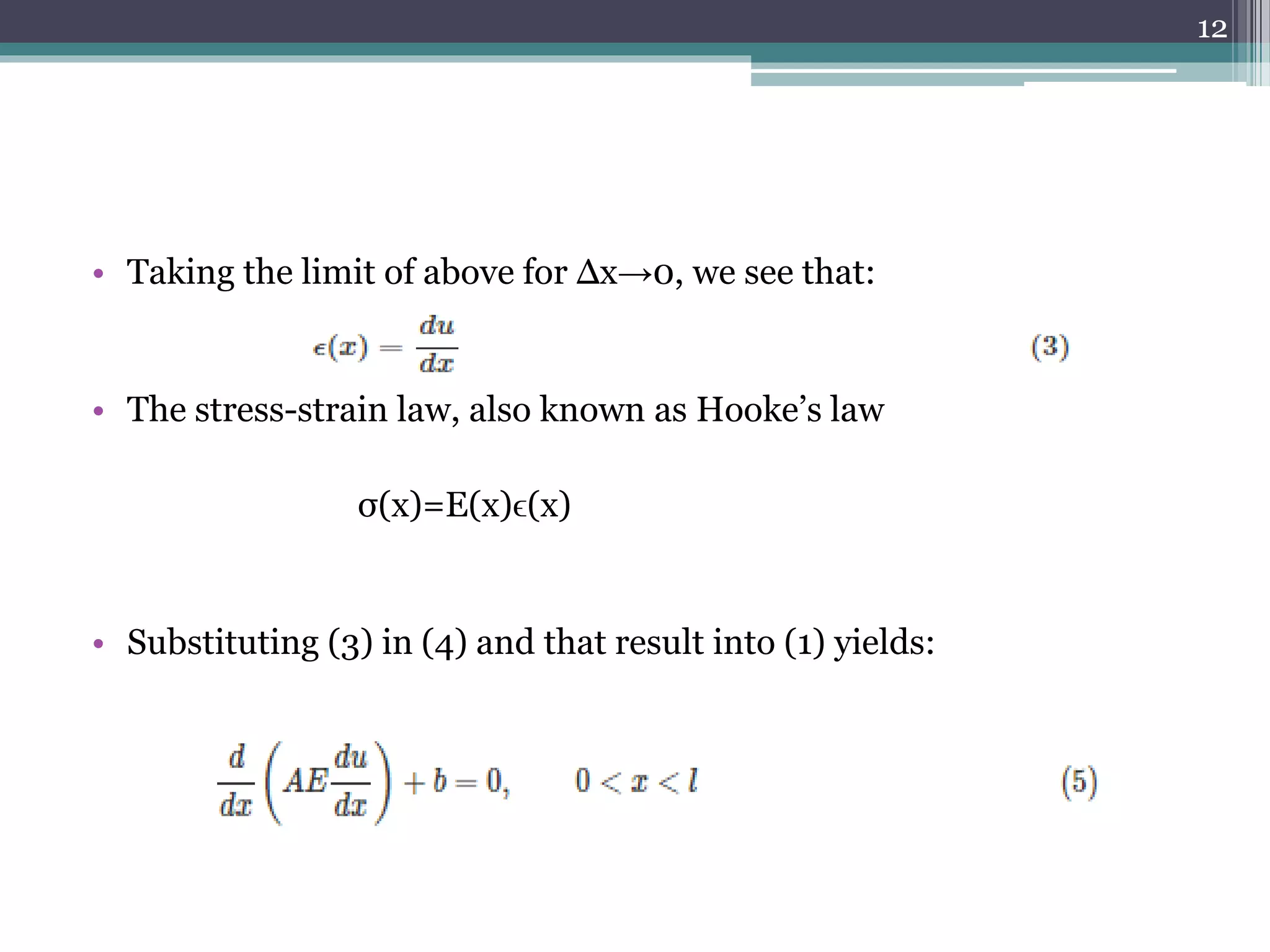
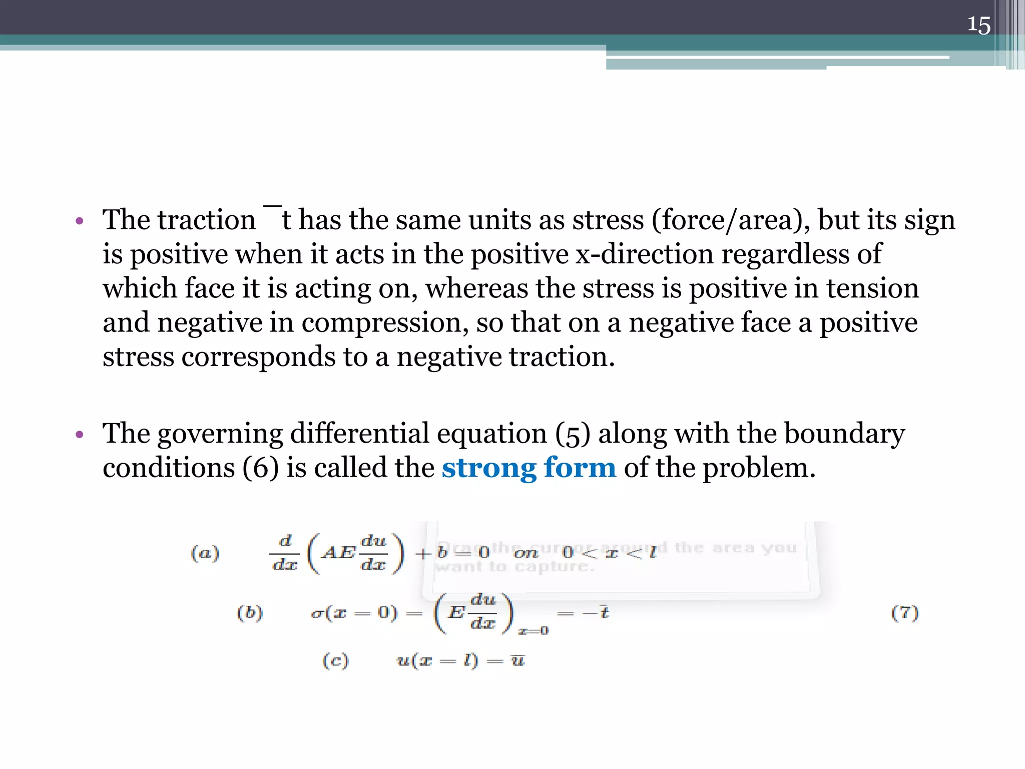
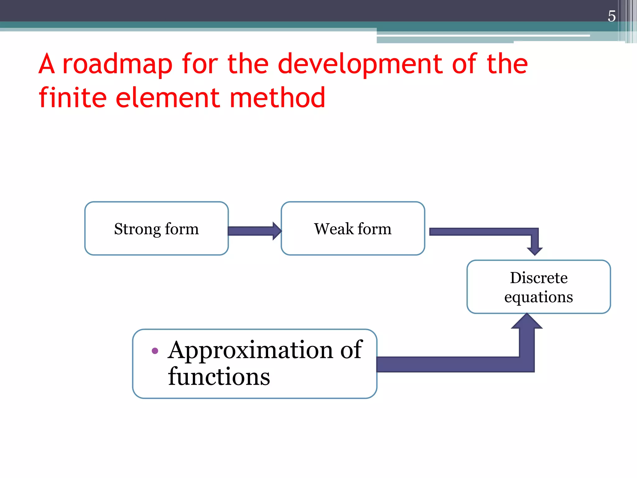
- The document discusses the strong form and weak form for analyzing an axially loaded elastic bar. - The strong form consists of the governing differential equations and boundary conditions. For the bar example, this includes the equilibrium equation and stress-strain relationships. - The weak form is developed by multiplying the strong form equations by a weight function, integrating over the domain, and using integration by parts. This transfers the derivatives from the displacement variable to the weight function. 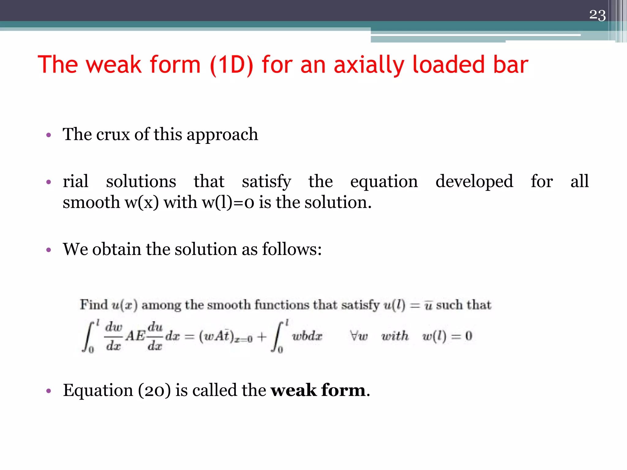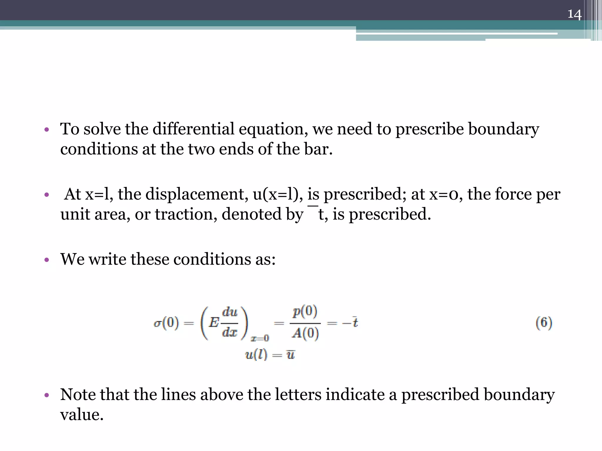- For the bar example, the weak form results in an equation that must hold for all admissible weight functions, and naturally includes the traction boundary conditions while only requiring the trial solutions to satisfy the essential displacement boundary conditions.

1. Strong form and Weak form
- Dharmendra Vankar
(19565001)
1

2. Strong form and Weak form
(Explanation through examples of a bar)
• To demonstrate the basic steps in formulating the “strong and weak
forms”, we will consider axially loaded elastic bars and heat
conduction problems in one dimension.
• The strong forms for these problems will be developed along with
the boundary conditions.
• Then we will develop weak forms for these problems and show that
they are equivalent to the strong forms.
2

3. The Weak form
• A weak form is defined to be a weighted integral statement of a
differential equation in which the differentiation is transferred from
the dependent variable to the weight function such that all natural
boundary conditions of the problem are also included in the integral
statement.
Main characteristics of weak formulation are
• (1) It requires weaker continuity of the dependent variable, and for
self-adjoint equations it always results in a symmetric coefficient
matrix.
• (2) the natural boundary conditions of the problem are included in
the weak form, and therefore the approximate solution is required
to satisfy only the essential boundary conditions of the problem.
3

4. The strong form
• The strong form consists of the governing equations and the
boundary conditions for a physical system.
• The governing equations are usually partial differential equations,
but in the one-dimensional case they become ordinary differential
equations.
4

5. A roadmap for the development of the
finite element method
5
Strong form Weak form
Discrete
equations
• Approximation of
functions

6. The strong form for an axially loaded bar
6
• Consider the static response of an elastic bar with variable cross section as
shown in the picture above

7. The strong form for an axially loaded bar
• This is an example of a problem in linear stress analysis or linear
elasticity
• where we seek to find the stress distribution σ(x) in the bar.
• The stress will result from the deformation of the body, which is
characterized by the displacement of points in the body, u(x).
• This displacement implies a strain denoted by ϵ(x).
• the body is subjected to a body force or distributed
loading b(x) (units are force per length)
7

8. • In addition, we can describe the body force which could be due to
gravity.
• Furthermore, loads can be prescribed at the ends of the bar.
• where the displacement is not prescribed → these loads are
called tractions and denoted by ¯t (units are force per area).
• multiplied with an area give us the applied force).
8

9. The bar must satisfy the following conditions
1. Equilibrium must be fulfilled
2. Stress-Strain law must be satisfied. σ(x)=E(x)ϵ(x)
3. Displacement field must be compatible
4. Strain-Displacement equations must be satisfied
9

10. • The differential equation of this bar can be obtained from
equilibrium of external forces b(x) as well as the internal
forces p(x) acting on the body in the axial direction (along x-axis).
• Summing the forces in x-direction:
Rearranging the terms:
10

11. • The limit of this equation with Δx→0 makes the first term the
derivative dp/dx and the second term becomes b(x). So we can
write:
(1)
• This equation expresses the equilibrium equation in terms of the
internal force p. Stress is defined as:
• The strain-displacement equation is obtained by:
11

12. • Taking the limit of above for Δx→0, we see that:
• The stress-strain law, also known as Hooke’s law
σ(x)=E(x)ϵ(x)
• Substituting (3) in (4) and that result into (1) yields:
12

13. • Equation (5) is a second-order ordinary differential equation.
• u(x) is the dependent variable, which is the unknown function, and x
the independent variable.
•
• Equation (5) is a specific form of equation (1). Equation (1) applies both
linear and nonlinear materials whereas (5) assumes linearity in the
definition of the strain (3) and stress-strain law (4)
• Compatibility is satisfied by requiring the displacement to be
continuous.
13

14. • To solve the differential equation, we need to prescribe boundary
conditions at the two ends of the bar.
• At x=l, the displacement, u(x=l), is prescribed; at x=0, the force per
unit area, or traction, denoted by ¯t, is prescribed.
• We write these conditions as:
• Note that the lines above the letters indicate a prescribed boundary
value.
14

15. • The traction ¯t has the same units as stress (force/area), but its sign
is positive when it acts in the positive x-direction regardless of
which face it is acting on, whereas the stress is positive in tension
and negative in compression, so that on a negative face a positive
stress corresponds to a negative traction.
• The governing differential equation (5) along with the boundary
conditions (6) is called the strong form of the problem.
15

16. The weak form (1D) for an axially loaded bar
• To develop the finite element formulation, the partial differential
equations must be restated in an integral form called the weak
form.
• The weak form and the strong form are equivalent! In stress
analysis the weak form is called the principle of virtual work..
• We start by multiplying the governing equation (7a) and the traction
boundary condition (7b) by an arbitrary function w(x) and
integrating over the domains on which they hold: for the governing
equation.
16

17. The weak form (1D) for an axially loaded bar
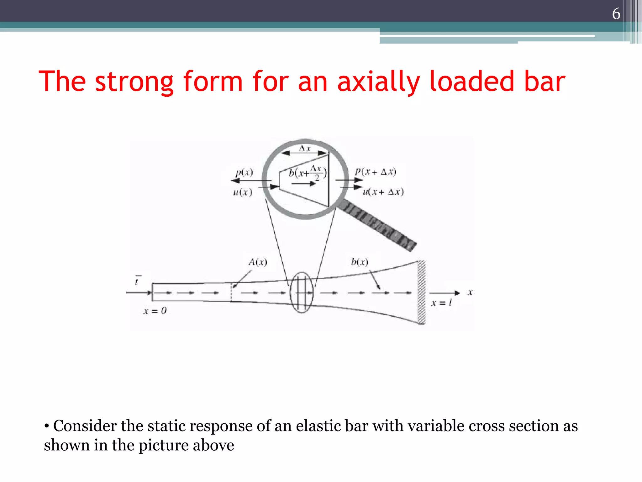
• the pertinent domain is [0,l]
• For the traction boundary, it is the cross-sectional area at x = 0 (no
integral needed since this condition only holds only at a point but
we multiply it with A).
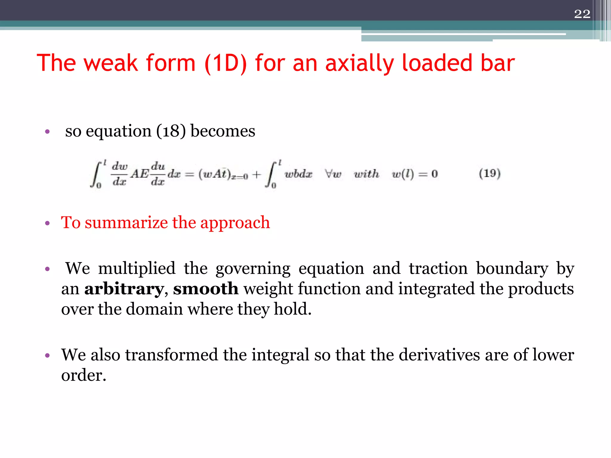
• The results are:
• The function w is called weight function or test function.
17

18. The weak form (1D) for an axially loaded bar
In the, ∀w denotes that w(x) is an arbitrary function, i.e. (13) has to
hold for all functions w(x).
• Arbitrariness of the weight function is crucial for the weak form.
• Otherwise the strong form is NOT equivalent to the weak form.
• We did not enforce the boundary condition on the displacement in
(13) by the weight function.
• It will be seen that it is easy to construct trial solutions u(x) that
satisfy this boundary condition.
18

19. The weak form (1D) for an axially loaded bar
We will also see that all weight functions satisfy
w(l)=0...................................................(14)
In solving the weak form, a set of admissible solutions u(x) that
satisfy certain conditions is considered (also called trial
solutions or candidate solutions).
We rewrite (13a) in an equivalent form:
19

20. The weak form (1D) for an axially loaded bar
• Applying integration by parts on equation (15):
• Using (16),equation (15) can be written as:
• We note that by the stress-strain law and strain-displacement
equations, the underscored boundary term is the stress σ:
20

21. The weak form (1D) for an axially loaded bar
• The first term in equation (18) vanishes since we assumed w(l)=0
• for that reason is it useful to construct weight functions that vanish
on prescribed displacement boundaries.
• Though the term looks insignificant, it would lead to loss of
symmetry in the final equation.
• Form (13b), we can see that the second term equals (wA¯t)x=0,
21

22. The weak form (1D) for an axially loaded bar
• so equation (18) becomes
• To summarize the approach
• We multiplied the governing equation and traction boundary by
an arbitrary, smooth weight function and integrated the products
over the domain where they hold.
• We also transformed the integral so that the derivatives are of lower
order.
22

23. The weak form (1D) for an axially loaded bar
• The crux of this approach
• rial solutions that satisfy the equation developed for all
smooth w(x) with w(l)=0 is the solution.
• We obtain the solution as follows:
• Equation (20) is called the weak form.
23

24. The weak form (1D) for an axially loaded bar
• The name states that solutions to the weak form do not need to be as
smooth as solutions of the strong form.
• You have to keep in mind that the solution satisfying equation (20) is
also the solution of the strong counterpart of this equation.
• Also remember that the trial solutions u(x) must satisfy
the displacement boundary conditions.
• This is an essential property of the trial solutions and that is why we
call those boundary conditions essential boundary conditions.
• The traction boundary conditions emanate naturally from equation
(20) which means that the trial solutions do not need to be constructed
to satisfy the traction boundary condition.
• These boundary conditions are therefore called natural boundary
conditions.
24

25. The weak form (1D) for an axially loaded bar
• A trial solution that is smooth AND satisfies the essential
boundary conditions is called admissible.
• A weight function that is smooth AND vanishes on essential
boundaries is admissible.
• When weak forms are used to solve a problem, the trial solutions
and weight functions must be admissible.
• Also notice that equation (20) is symmetric in w and u which will
lead to a symmetric stiffness matrix.
• The highest order derivative that appears in this equation is of first
order!
25

26. 26