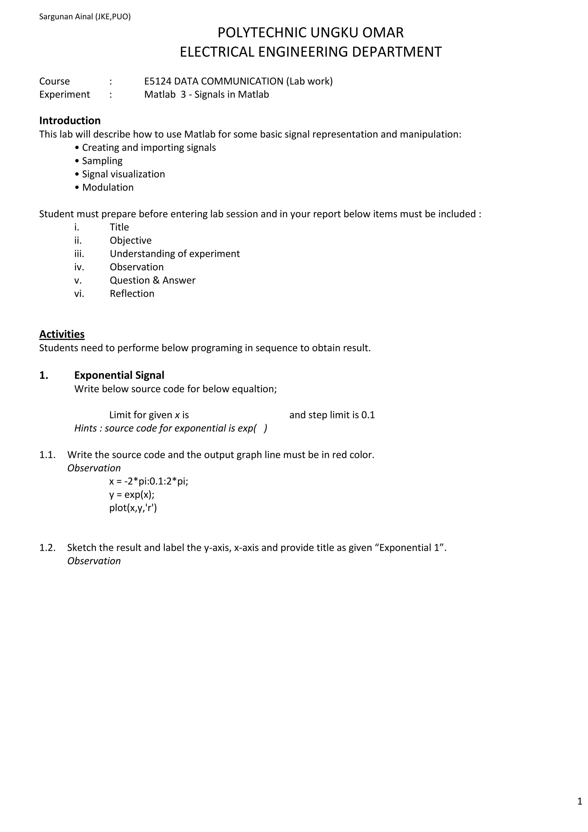
Sargunan Ainal (JKE,PUO)

                                      POLYTECHNIC UNGKU OMAR
                                 ELECTRICAL ENGINEERING DEPARTMENT
Course            :        E5124 DATA COMMUNICATION (Lab work)
Experiment        :        Matlab 3 - Signals in Matlab

Introduction
This lab will describe how to use Matlab for some basic signal representation and manipulation:
         • Creating and importing signals
         • Sampling
         • Signal visualization
         • Modulation

Student must prepare before entering lab session and in your report below items must be included :
       i.      Title
       ii.     Objective
       iii.    Understanding of experiment
       iv.     Observation
       v.      Question & Answer
       vi.     Reflection


Activities
Students need to performe below programing in sequence to obtain result.

1.       Exponential Signal
         Write below source code for below equaltion;

                  Limit for given x is                     and step limit is 0.1
         Hints : source code for exponential is exp( )

1.1.   Write the source code and the output graph line must be in red color.
       Observation
                x = -2*pi:0.1:2*pi;
                y = exp(x);
                plot(x,y,'r')


1.2.   Sketch the result and label the y-axis, x-axis and provide title as given “Exponential 1”.
       Observation


                                                                                                     1
Sargunan Ainal (JKE,PUO)

1.3.   Now, writesource code to produce resultfor below equation.

                  Limit for given x is          and step limit is 0.1

         Observation
                x = 0:0.1:10;
                y = exp(x);
                plot(x,y,'r')


1.4.   Now plot both result in single Figure outcome (use subplot).
       Hints : use suubplot and label with title your output
       Observation


1.5.   Write the source code used and state your comparison.
       Observation


                                                                        2
Sargunan Ainal (JKE,PUO)


2. Pulse Amplitude Modulation (PAM)
    Procedure:
    a. Launch the Matlab program (click Matlab icon)
    b. Click tab, FILE NEW M-FILE . New window screen will pop out and it looks like notepad. Use it to write below
        source code.
                % Name : fill in your name
                % Reg No. : fill in your reg. no
                % Class : fill in class
                % Sampling frequency 24000 Hz
                % Symbol time interval [s].
                T = 1/8000;
                Fs = 24000;
                % Time vector (sampling intervals) , -5T<1/Fs>5T
                t = -5T:1/Fs:5T;
                % Otherwise, the denominator would be zero at t=0 (or manually set “p(t=0)=1”)
                t = t+1e-10;
                % Roll-off factor
                alfa = 0.5;
                p = (sin(pi*t/T)./(pi*t/T)).*(cos(alfa*pi*t/T)./(1-(2*alfa*t/T).^2));
                % Raised-Cosine FIR filter
                clf;
                plot(ts,p)
                hold on;
                stem(ts,p)
                hold off;

    c. Save the written source code using “PAM.m” name.
    d. At the same window, click tab DEBUG RUN.
       Now the source code will execute and produce result. Check the Matlab main window at Command Window
       prompt, there will be error occurance.
    e. What are the errors and how you solve it?
       Observation
                      t = -5T:1/Fs:5T;        t = -5*T:1/Fs:5*T;
                      plot(ts,p)              plot(t,p);
                      stem(ts,p)              stem(t,p);


    f.   Label x-axis with Time, y-axis with Amplitude and title as PAM Spectrum and state observation
         Observation


    g. Now, change the below parameter
         i.   T = 1/8000 with T=1/2000, record your observation


                                                                                                                  3
Sargunan Ainal (JKE,PUO)
                  Observation


           ii.    Reset the T value to original and change the sampling frequency to 240kHz, record your observation


    h. Why there is clf command in the program and explain it.

         clf deletes from the current figure all graphics objects whose handles are not hidden

    i.   Set back samapling frequency 240kHz to 24kHz. What will happen if the hold on is removed?
         Observation


                                                                                                                       4
Sargunan Ainal (JKE,PUO)
3. Analogue to Digital
3.1.   Wite this source code in M-File.

         n=[0:1/44100:1];
         sine1=sin(2*pi*10.*n)
         sine2=0.5*sin(2*pi*30.*n)
         sine3=0.25*sin(2*pi*50.*n)
         sine4=0.125*sin(2*pi*70.*n)
         sine5=0.0625*sin(2*pi*90.*n)
         figure(1)
         subplot(5,1,1);
         plot(n,sine1);
         subplot(5,1,1);
         plot(n,sine1+sine2);
         plot(n,sine1+sine2+sine3)
         subplot(5,1,4);
         plot(n,sine1+sine2+sine3+sine4);
         subplot(5,1,4)
         plot(n,sine1+sine2+sine3+sine4+sine5)

3.2.   Save the written source code using “ADC” name.
3.3.   Execute RUN command.
3.4.   Now the source code will execute and produce result. Check the Matlab main window at Command Window
       prompt.
3.5.   What are the errors and state your solutions.
       Observation


3.6.   Label x-axis with Number of sample, y-axis with Amplitude and title as Analogue to Digital for each graphical output.
       Observation


3.7.   Now, change the below parameter
       a) sine5=0.0625*sin(2*pi*90.*n) to sine5=0.0625*sin(2*pi*190.*n), record your observation
          Observation


       b) Reset the sine5 value to original and add another one more graph output in your display. Record your
          observation and there will be minor changes between graph sine5 and the new graph.
          Observation


                                                                                                                           5
Sargunan Ainal (JKE,PUO)
3.8.   Remain the 3.7. result.
3.9.   What is the meaning of subplot (5,1,4)?

       ____________________________________________________________________________________

       ____________________________________________________________________________________


3.10. Convert your 6x1 matrices to other form of matrices which more convinent to application.
      Observation


                                                                                                 6

Matlab 3

  • 1.
    Sargunan Ainal (JKE,PUO) POLYTECHNIC UNGKU OMAR ELECTRICAL ENGINEERING DEPARTMENT Course : E5124 DATA COMMUNICATION (Lab work) Experiment : Matlab 3 - Signals in Matlab Introduction This lab will describe how to use Matlab for some basic signal representation and manipulation: • Creating and importing signals • Sampling • Signal visualization • Modulation Student must prepare before entering lab session and in your report below items must be included : i. Title ii. Objective iii. Understanding of experiment iv. Observation v. Question & Answer vi. Reflection Activities Students need to performe below programing in sequence to obtain result. 1. Exponential Signal Write below source code for below equaltion; Limit for given x is and step limit is 0.1 Hints : source code for exponential is exp( ) 1.1. Write the source code and the output graph line must be in red color. Observation x = -2*pi:0.1:2*pi; y = exp(x); plot(x,y,'r') 1.2. Sketch the result and label the y-axis, x-axis and provide title as given “Exponential 1”. Observation 1
  • 2.
    Sargunan Ainal (JKE,PUO) 1.3. Now, writesource code to produce resultfor below equation. Limit for given x is and step limit is 0.1 Observation x = 0:0.1:10; y = exp(x); plot(x,y,'r') 1.4. Now plot both result in single Figure outcome (use subplot). Hints : use suubplot and label with title your output Observation 1.5. Write the source code used and state your comparison. Observation 2
  • 3.
    Sargunan Ainal (JKE,PUO) 2.Pulse Amplitude Modulation (PAM) Procedure: a. Launch the Matlab program (click Matlab icon) b. Click tab, FILE NEW M-FILE . New window screen will pop out and it looks like notepad. Use it to write below source code. % Name : fill in your name % Reg No. : fill in your reg. no % Class : fill in class % Sampling frequency 24000 Hz % Symbol time interval [s]. T = 1/8000; Fs = 24000; % Time vector (sampling intervals) , -5T<1/Fs>5T t = -5T:1/Fs:5T; % Otherwise, the denominator would be zero at t=0 (or manually set “p(t=0)=1”) t = t+1e-10; % Roll-off factor alfa = 0.5; p = (sin(pi*t/T)./(pi*t/T)).*(cos(alfa*pi*t/T)./(1-(2*alfa*t/T).^2)); % Raised-Cosine FIR filter clf; plot(ts,p) hold on; stem(ts,p) hold off; c. Save the written source code using “PAM.m” name. d. At the same window, click tab DEBUG RUN. Now the source code will execute and produce result. Check the Matlab main window at Command Window prompt, there will be error occurance. e. What are the errors and how you solve it? Observation t = -5T:1/Fs:5T; t = -5*T:1/Fs:5*T; plot(ts,p) plot(t,p); stem(ts,p) stem(t,p); f. Label x-axis with Time, y-axis with Amplitude and title as PAM Spectrum and state observation Observation g. Now, change the below parameter i. T = 1/8000 with T=1/2000, record your observation 3
  • 4.
    Sargunan Ainal (JKE,PUO) Observation ii. Reset the T value to original and change the sampling frequency to 240kHz, record your observation h. Why there is clf command in the program and explain it. clf deletes from the current figure all graphics objects whose handles are not hidden i. Set back samapling frequency 240kHz to 24kHz. What will happen if the hold on is removed? Observation 4
  • 5.
    Sargunan Ainal (JKE,PUO) 3.Analogue to Digital 3.1. Wite this source code in M-File. n=[0:1/44100:1]; sine1=sin(2*pi*10.*n) sine2=0.5*sin(2*pi*30.*n) sine3=0.25*sin(2*pi*50.*n) sine4=0.125*sin(2*pi*70.*n) sine5=0.0625*sin(2*pi*90.*n) figure(1) subplot(5,1,1); plot(n,sine1); subplot(5,1,1); plot(n,sine1+sine2); plot(n,sine1+sine2+sine3) subplot(5,1,4); plot(n,sine1+sine2+sine3+sine4); subplot(5,1,4) plot(n,sine1+sine2+sine3+sine4+sine5) 3.2. Save the written source code using “ADC” name. 3.3. Execute RUN command. 3.4. Now the source code will execute and produce result. Check the Matlab main window at Command Window prompt. 3.5. What are the errors and state your solutions. Observation 3.6. Label x-axis with Number of sample, y-axis with Amplitude and title as Analogue to Digital for each graphical output. Observation 3.7. Now, change the below parameter a) sine5=0.0625*sin(2*pi*90.*n) to sine5=0.0625*sin(2*pi*190.*n), record your observation Observation b) Reset the sine5 value to original and add another one more graph output in your display. Record your observation and there will be minor changes between graph sine5 and the new graph. Observation 5
  • 6.
    Sargunan Ainal (JKE,PUO) 3.8. Remain the 3.7. result. 3.9. What is the meaning of subplot (5,1,4)? ____________________________________________________________________________________ ____________________________________________________________________________________ 3.10. Convert your 6x1 matrices to other form of matrices which more convinent to application. Observation 6