This document provides a technical explanation of simulating multirate digital signal processing (DSP) systems using MATLAB's Signal Processing Toolbox. It details the command line functions for generating bandlimited signals, performing upsampling and downsampling, and implementing lowpass filtering to avoid aliasing. Additionally, examples illustrate the differences between using command line functions and Simulink with the DSP blockset for enhanced visualization and manipulation of the DSP systems.

1. Introduction 1
Multirate Sampling Simulation Using
MATLAB’s Signal Processing Toolbox
Introduction
This technical note explains how you can very easily use the command line functions available in
the MATLAB signal processing toolbox, to simulate simple multirate DSP systems. The focus
here is to be able to view in the frequency domain what is happening at each stage of a system
involving upsamplers, downsamplers, and lowpass filters. All computations will be performed
using MATLAB and the signal processing toolbox. These same building blocks are available in
Simulink via the DSP blockset. The DSP blockset allows better visualization of the overall sys-
tem, but is not available in the ECE general computing laboratory or on most personal systems. A
DSP block set example will be included here just so one can see the possibilities with the addi-
tional MATLAB tools.
Command Line Building Blocks
To be able to visualize the spectra in a multirate system we need the basic building blocks of
• Bandlimited signal generation; here we create a signal with a triangle shaped spectrum using
sinc()
• Integer upsampling and downsampling operations; here we use the signal processing tool-
box functions upsample() and downsample()
• Lowpass filtering for antialiasing and interpolation; here we use fir1()
• If we don’t care to examine the spectra between the antialiasing lowpass filter and the deci-
mator or between the upsampler and interpolation filter, we can use combination functions
such as decimate(), interpolate(), and resample()
Signal Generation
In a theoretical discussion of sampling theory it is common place to represent the signal of interest
as having a triangular shaped Fourier spectrum. Another common signal type is one or more dis-
crete-time sinusoids. We know that
(1)
where
ωcnsin
πn
-----------------
ω
2ωc
---------
 
 
∏↔
F
x
W 2⁄W 2⁄–
1x
W
-----
 
 
∏ = W

2. ECE 5650/4650 Simulation with MATLAB
Command Line Building Blocks 2
A triangle can be obtained in the frequency domain by noting that
(2)
The periodic convolution on the right-side of (2) yields
where is the spectral bandwidth (single-sided or lowpass) in normalized frequency units. It
then follows that for a unit height spectrum we have the transform pair
(3)
where
Using the sinc( ) function in MATLAB, which is defined as
(4)
we can write (3) as
(5)
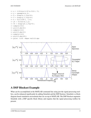
Creating a triangular spectrum signal in MATLAB just requires delaying the signal in samples so
that both tails can be represented in a causal simulation, e.g.,
>> n = 0:1024;
>> x = 1/4*sinc(1/4*(n-512)).^2; % set peak of signal to center of interval
>> f = -1:1/512:1; % create a custom frequency axis for spectral plotting
>> X = freqz(x,1,2*pi*f); %Compute the Fourier transform of x
>> plot(f,abs(X))
>> print -tiff -depsc multi1.eps
ωcn 2⁄( )sin
πn
-----------------------------
2
1
2π
------
ω θ–
ωc
-------------
 
  θ
ωc
------
 
 
∏∏ θd
π–
π
∫↔
F
ω
ωcω– c
ωc
2π
------ fc=
fc
2π
ωc
------
ωcn 2⁄( )sin
πn
-----------------------------
 
 
2
Λ
ω
ωc
------
 
 ↔
F
x
WW–
1
Λ
x
W
-----
 
  =
sinc x( )
πxsin
πx
--------------≡
fc sinc fcn( )[ ]
2
Λ
ω
2πfc
----------
 
 ↔
F

3. ECE 5650/4650 Simulation with MATLAB
Command Line Building Blocks 3
Consider a couple of more examples:
>> n = 0:1024;
>> x125 = 1/8*sinc(1/8*(n-512)).^2;
>> x5 = 1/2*sinc(1/2*(n-512)).^2;
>> f = -1:1/512:1;
>> X125 = freqz(x125,1,2*pi*f);
>> X5 = freqz(x5,1,2*pi*f);
>> subplot(211)
>> plot(f,abs(X125))
>> subplot(212)
>> plot(f,abs(X5))
>> print -tiff -depsc multi2.eps
Upsample and Downsample
With a means to generate a signal having bandlimited spectra in place, we can move on to the
upsampling and downsampling operations. The signal processing toolbox has dedicated functions
for doing this operation, although they are actually quite easy to write yourself.
>> help downsample
−1 −0.8 −0.6 −0.4 −0.2 0 0.2 0.4 0.6 0.8 1
0
0.2
0.4
0.6
0.8
1
Normalized Frequency
ω
2π
------
X e
jω
( )
fc 0.25 or ωc
π
2
---= =
−1 −0.8 −0.6 −0.4 −0.2 0 0.2 0.4 0.6 0.8 1
0
0.5
1
−1 −0.8 −0.6 −0.4 −0.2 0 0.2 0.4 0.6 0.8 1
0
0.5
1
Normalized Frequency
ω
2π
------
X e
jω
( )
X e
jω
( )
ωc
π
4
---=
ωc π=

4. ECE 5650/4650 Simulation with MATLAB
Command Line Building Blocks 4
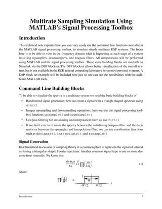
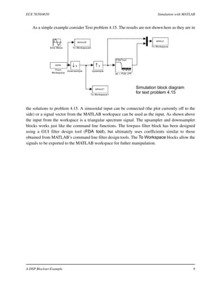
DOWNSAMPLE Downsample input signal.
DOWNSAMPLE(X,N) downsamples input signal X by keeping every
N-th sample starting with the first. If X is a matrix, the
downsampling is done along the columns of X.
DOWNSAMPLE(X,N,PHASE) specifies an optional sample offset.
PHASE must be an integer in the range [0, N-1].
See also UPSAMPLE, UPFIRDN, INTERP, DECIMATE, RESAMPLE.
>> help upsample
UPSAMPLE Upsample input signal.
UPSAMPLE(X,N) upsamples input signal X by inserting
N-1 zeros between input samples. X may be a vector
or a signal matrix (one signal per column).
UPSAMPLE(X,N,PHASE) specifies an optional sample offset.
PHASE must be an integer in the range [0, N-1].
See also DOWNSAMPLE, UPFIRDN, INTERP, DECIMATE, RESAMPLE.
These functions will be used in examples that follow.
Filtering
To implement a simple yet effective lowpass filter to prevent aliasing in a downsampler and inter-
polation in an upsampler, we can use the function fir1() which designs linear phase FIR filters
using a windowed sinc function.
>> help fir1
FIR1 FIR filter design using the window method.
B = FIR1(N,Wn) designs an N'th order lowpass FIR digital filter
and returns the filter coefficients in length N+1 vector B.
The cut-off frequency Wn must be between 0 < Wn < 1.0, with 1.0
corresponding to half the sample rate. The filter B is real and
has linear phase. The normalized gain of the filter at Wn is
-6 dB.
More help beyond this, but this is the basic LPF design interface
The filter design functions use half sample rate normalized frequencies:
ω
f′
π 2π
10
Input on f′ axis
π M⁄
1 M⁄
To get this,
enter this

5. ECE 5650/4650 Simulation with MATLAB
System Simulation 5
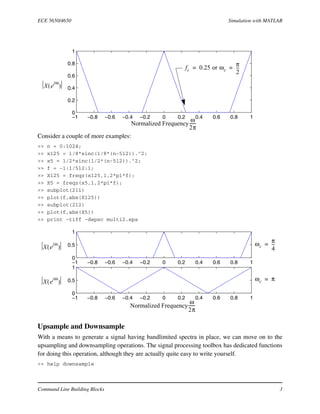
To design a lowpass filter FIR filter having 128 coefficients and a cutoff frequency of ,
we simply type
>> h = fir1(128-1,1/3); % Input cutoff as 2*fc, where fc = wc/(2pi)
>> freqz(h,1,512,1)
>> print -tiff -depsc multi3.eps
System Simulation
To keep things simple we will consider just simple decimator and interpolator systems.
A Simple Decimation Example
In the above system we will consider the pure decimator and the decimator with lowpass prefilter-
ing. Two different values of M will be considered.
As a first example we pass directly into an decimator with a signal having
( ).
>> n = 0:1024;
ωc π 3⁄=
0 0.05 0.1 0.15 0.2 0.25 0.3 0.35 0.4 0.45 0.5
−6000
−4000
−2000
0
Frequency (Hz)
Phase(degrees)
0 0.05 0.1 0.15 0.2 0.25 0.3 0.35 0.4 0.45 0.5
−80
−60
−40
−20
0
Frequency (Hz)
Magnitude(dB)
Mx n[ ] y n[ ]
Lowpass
ωc
π
M
-----=
ω
ωNω– N
1X e
jω
( )
Bypass LPF
M 2=
ωN π 2⁄= fN 1 4⁄=

6. ECE 5650/4650 Simulation with MATLAB
System Simulation 6
>> x = 1/4*sinc(1/4*(n-512)).^2;
>> y = downsample(x,2);
>> f = -1:1/512:1;
>> X = freqz(x,1,2*pi*f);
>> Y = freqz(y,1,2*pi*f);
>> plot(f,abs(X))
>> subplot(211)
>> plot(f,abs(X))
>> subplot(212)
>> plot(f,abs(Y))
>> print -tiff -depsc multi4.eps
• The results are exactly as we would expect
Now, use the same signal except with . First without the prefilter, and then include it to
avoid aliasing.
>> n = 0:1024;
>> x = 1/4*sinc(1/4*(n-512)).^2;
>> xf = filter(h,1,x);
>> yf = downsample(xf,3);
>> ynf = downsample(x,3);
>> X = freqz(x,1,2*pi*f);
>> Xf = freqz(xf,1,2*pi*f);
>> Yf = freqz(yf,1,2*pi*f);
>> Ynf = freqz(ynf,1,2*pi*f);
>> subplot(411)
−1 −0.8 −0.6 −0.4 −0.2 0 0.2 0.4 0.6 0.8 1
0
0.5
1
−1 −0.8 −0.6 −0.4 −0.2 0 0.2 0.4 0.6 0.8 1
0
0.2
0.4
0.6
0.8
Normalized Frequency
ω
2π
------
X e
jω
( )
Y e
jω
( )
L 2 Decimation, No Prefilter=
No aliasing
problems
M 3=

7. ECE 5650/4650 Simulation with MATLAB
System Simulation 7
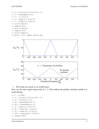
>> plot(f,abs(X))
>> subplot(412)
>> plot(f,abs(Ynf))
>> subplot(413)
>> plot(f,abs(Xf))
>> subplot(414)
>> plot(f,abs(Yf))
>> print -tiff -depsc multi5.eps
A Simple Interpolation System
In the above system we will consider the pure upsampler and the upsampler followed by a low-
pass interpolation filter. Let and the signal have ( ).
>> n = 0:1024;
−1 −0.8 −0.6 −0.4 −0.2 0 0.2 0.4 0.6 0.8 1
0
0.5
1
−1 −0.8 −0.6 −0.4 −0.2 0 0.2 0.4 0.6 0.8 1
0
0.2
0.4
−1 −0.8 −0.6 −0.4 −0.2 0 0.2 0.4 0.6 0.8 1
0
0.5
1
−1 −0.8 −0.6 −0.4 −0.2 0 0.2 0.4 0.6 0.8 1
0
0.2
0.4
Normalized Frequency
ω
2π
------
X e
jω
( )
Yf e
jω
( )
Xf e
jω
( )
Ynf e
jω
( )
Aliasing Aliasing
Unfiltered
Input
Filtered
Input
Down by 3
w/o Filter
Output
Down by 3
with Filter
OutputShould be 0
but filter is
not ideal
Lowpass
ωc
π
3
---=3 yr n[ ]x n[ ]
yu n[ ]
ω
ωNω– N
1X e
jω
( )
L 3= ωN π 2⁄= fN 1 4⁄=

8. ECE 5650/4650 Simulation with MATLAB
A DSP Blockset Example 8
>> x = 1/4*sinc(1/4*(n-512)).^2;
>> y = upsample(x,3);
>> X = freqz(x,1,2*pi*f);
>> Y = freqz(y,1,2*pi*f);
>> h = fir1(128-1, 1/3);
>> yf = filter(h,1,y);
>> Yf = freqz(yf,1,2*pi*f);
>> subplot(311)
>> plot(f,abs(X))
>> subplot(312)
>> plot(f,abs(Y))
>> subplot(313)
>> plot(f,abs(Yf))
>> print -tiff -depsc multi6.eps
A DSP Blockset Example
What can be accomplished at the MATLAB command line using just the signal processing tool-
box, can be enhanced significantly by adding Simulink and the DSP blockset. Simulink is a block
diagram based simulation environment that sits on top of MATLAB. The DSP blockset augments
Simulink with a DSP specific block library and requires that the signal processing toolbox be
present.
−1 −0.8 −0.6 −0.4 −0.2 0 0.2 0.4 0.6 0.8 1
0
0.5
1
−1 −0.8 −0.6 −0.4 −0.2 0 0.2 0.4 0.6 0.8 1
0
0.5
1
−1 −0.8 −0.6 −0.4 −0.2 0 0.2 0.4 0.6 0.8 1
0
0.5
1
Normalized Frequency
ω
2π
------
X e
jω
( )
Yf e
jω
( )
Y e
jω
( )
Images removed
by lowpass filter
Input
Spectrum
Upsampled
by 3 Input
Interp.
Upsample
Output

9. ECE 5650/4650 Simulation with MATLAB
A DSP Blockset Example 9
As a simple example consider Text problem 4.15. The results are not shown here as they are in
the solutions to problem 4.15. A sinusoidal input can be connected (the plot currently off to the
side) or a signal vector from the MATLAB workspace can be used as the input. As shown above
the input from the workspace is a triangular spectrum signal. The upsampler and downsampler
blocks works just like the command line functions. The lowpass filter block has been designed
using a GUI filter design tool (FDA tool), but ultimately uses coefficients similar to those
obtained from MATLAB’s command line filter design tools. The To Workspace blocks allow the
signals to be exported to the MATLAB workspace for futher manipulation.
FDATool
wc = Pi/8 LPF
3
Upsample
simout2
To Workspace2
simout1
To Workspace1
simout
To Workspace
Sine Wave
simin
From
Workspace
3
Downsample
Simulation block diagram
for text problem 4.15