This document contains MATLAB code and output for generating and analyzing various types of discrete-time signals including unit sample sequences, exponential sequences, sinusoidal sequences, random sequences, and complex signals like amplitude modulation. The document contains MATLAB programs to generate these signals and questions about modifying the programs and analyzing properties of the generated signals.

1. Name :
Section :
Laboratory Exercise 1
DISCRETE-TIME SIGNALS: TIME-DOMAIN REPRESENTATION
1.1 GENERATION OF SEQUENCES
Project 1.1 Unit sample and unit step sequences
A copy of Program P1_1 is given below.
% Program P1_1
% Generation of a Unit Sample Sequence
clf;
% Generate a vector from -10 to 20
n = -10:20;
% Generate the unit sample sequence
u = [zeros(1,10) 8 zeros(1,20)];
% Plot the unit sample sequence
% stem para funciones discretas
stem(n,u);
xlabel('Time index n');ylabel('Amplitude');
title('Unit Sample Sequence');
axis([-10 20 0 1.2]);
Answers :
Q1.1 The unit sample sequence u[n] generated by running Program P1_1 is shown
below:
Q1.2 The purpose of clf com mand is – The screen is cleaned.
The purpose of axis com mand is – this activates the axis “x” and “y”
The purpose of title com mand is –this puts title in the graphics.
1

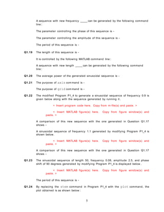
2. The purpose of xlabel com mand is – this puts legend in the axis “x”.
The purpose of ylabel com mand is – this puts legend in the axis “x”.
Q1.3 The modified Program P1_1 to generate a delayed unit sample sequence ud[n]
with a delay of 11 samples is given below along with the sequence generated by
running this program .
% Program P1_1
% Generation of a Unit Sample Sequence
clf;
% Generate a vector from -10 to 20
n = -10:20;
% Generate the unit sample sequence
ud = [zeros(1,21) 1 zeros(1,9) ];
% Plot the unit sample sequence
% stem para funciones discretas
stem(n,ud);
xlabel('Time index n');ylabel('Amplitude');
title('Unit Sample Sequence');
axis([-10 20 0 1.2]);
Q1.4 The modified Program P1_1 to generate a unit step sequence s[n] is given below
along with the sequence generated by running this program .
% Program P1_1
% Generation of a Unit Sample Sequence
clf;
% Generate a vector from -10 to 20
n = -10:20;
% Generate the unit sample sequence
s = [zeros(1,10) ones(1,21) ];
2

3. % Plot the unit sample sequence
% stem para funciones discretas
stem(n,s);
xlabel('Time index n');ylabel('Amplitude');
title('Unit Sample Sequence');
axis([-10 20 0 1.2]);
Q1.5 The modified Program P1_1 to generate a unit step sequence sd[n] with an ad-
vance of 7 samples is given below along with the sequence generated by running
this program .
< Insert program code here. Copy from m-file(s) and paste. >
< Insert MATLAB figure(s) here. Copy from figure window(s) and
paste. >
Project 1.2 Exponential signals
A copy of Programs P1_2 and P1_3 are given below .
< Insert program code here. Copy from m-file(s) and paste. >
Answers:
Q1.6 The complex- valued exponential sequence generated by running Program P1_2 is
shown below :
< Insert MATLAB figure(s) here. Copy from figure window(s) and
paste. >
Q1.7 The parameter controlling the rate of growth or decay of this sequence is -
The parameter controlling the amplitude of this sequence is -
Q1.8 The result of changing the parameter c to (1/12)+(pi/6)*i is -
3

4. Q1.9 The purpose of the operator real is -
The purpose of the operator imag is -
Q1.10 The purpose of the command subplot is -
Q1.11 The real-valued exponential sequence generated by running Program P1_3 is
shown below :
< Insert MATLAB figure(s) here. Copy from figure window(s) and
paste. >
Q1.12 The parameter controlling the rate of growth or decay of this sequence is -
The parameter controlling the amplitude of this sequence is -
Q1.13 The difference between the arithmetic operators ^ and .^ is -
Q1.14 The sequence generated by running Program P1_3 with the parameter a changed
to 0.9 and the parameter K changed to 20 is shown below :
< Insert MATLAB figure(s) here. Copy from figure window(s) and
paste. >
Q1.15 The length of this sequence is -
It is controlled by the following MATLAB command line :
It can be changed to generate sequences with different lengths as follows (give an
example command line and the corresponding length) :
Q1.16 The energies of the real-valued exponential sequences x[n]generated in Q1.11
and Q1.14 and computed using the command sum are -
Project 1.3 Sinusoidal sequences
A copy of Program P1_4 is given below .
< Insert program code here. Copy from m-file(s) and paste. >
Answers:
Q1.17 The sinusoidal sequence generated by running Program P1_4 is displayed below .
< Insert MATLAB figure(s) here. Copy from figure window(s) and
paste. >
Q1.18 The frequency of this sequence is -
It is controlled by the following MATLAB command line :
4

5. A sequence with new frequency _____ can be generated by the following command
line :
The parameter controlling the phase of this sequence is -
The parameter controlling the amplitude of this sequence is -
The period of this sequence is -
Q1.19 The length of this sequence is -
It is controlled by the following MATLAB command line :
A sequence with new length _____ can be generated by the following command
line :
Q1.20 The average power of the generated sinusoidal sequence is -
Q1.21 The purpose of axis com mand is -
The purpose of grid com mand is -
Q1.22 The modified Program P1_4 to generate a sinusoidal sequence of frequency 0.9 is
given below along with the sequence generated by running it .
< Insert program code here. Copy from m-file(s) and paste. >
< Insert MATLAB figure(s) here. Copy from figure window(s) and
paste. >
A comparison of this new sequence with the one generated in Question Q1.17
shows -
A sinusoidal sequence of frequency 1.1 generated by modifying Program P1_4 is
shown below.
< Insert MATLAB figure(s) here. Copy from figure window(s) and
paste. >
A comparison of this new sequence with the one generated in Question Q1.17
shows -
Q1.23 The sinusoidal sequence of length 50, frequency 0.08, amplitude 2.5, and phase
shift of 90 degrees generated by modifying Program P1_4 is displayed below .
< Insert MATLAB figure(s) here. Copy from figure window(s) and
paste. >
The period of this sequence is -
Q1.24 By replacing the stem command in Program P1_4 with the plot command, the
plot obtained is as shown below :
5

6. < Insert MATLAB figure(s) here. Copy from figure window(s) and
paste. >
The difference between the new plot and the one generated in Question Q1.17 is -
Q1.25 By replacing the stem command in Program P1_4 with the stairs command the
plot obtained is as shown below :
% Program P1_4
% Generation of a sinusoidal sequence
n = 0:40;
f = 0.1;
phase = 0;
A = 1.5;
arg = 2*pi*f*n - phase;
x = A*cos(arg);
clf; % Clear old graph
stairs(n,x); % Plot the generated sequence
axis([0 40 -2 2]);
grid;
title('Sinusoidal Sequence');
xlabel('Time index n');
ylabel('Amplitude');
axis;
The difference between the new plot and those generated in Questions Q1.17 and
Q1.24 is -
Project 1.4 Random signals
Answers:
Q1.26 The MATLAB program to generate and display a random signal of length 100 with
elements uniformly distributed in the interval [–2, 2] is given below along with the
plot of the random sequence generated by running the program :
< Insert program code here. Copy from m-file(s) and paste. >
6

7. < Insert MATLAB figure(s) here. Copy from figure window(s) and
paste. >
Q1.27 The MATLAB program to generate and display a Gaussian random signal of length
75 with elements normally distributed with zero mean and a variance of 3 is given
below along with the plot of the random sequence generated by running the
program :
< Insert program code here. Copy from m-file(s) and paste. >
< Insert MATLAB figure(s) here. Copy from figure window(s) and
paste. >
Q1.28 The MATLAB program to generate and display five sample sequences of a random
sinusoidal signal of length 31
{X[n]} = {Acos(ωon + φ)}
where the amplitude A and the phase φ are statistically independent random
variables with uniform probability distribution in the range 0 ≤ A ≤ 4 for the
amplitude and in the range 0 ≤ φ ≤ 2π for the phase is given below. Also shown
are five sample sequences generated by running this program five different times .
< Insert program code here. Copy from m-file(s) and paste. >
< Insert MATLAB figure(s) here. Copy from figure window(s) and
paste. >
1.2 SIMPLE OPERATIONS ON SEQUENCES
Project 1.5 Signal Smoothing
A copy of Program P1_5 is given below .
% Program P1_5
% Signal Smoothing by Averaging
clf;
R = 51;
d = 0.8*(rand(R,1) - 0.5); % Generate random noise
m = 0:R-1;
s = 2*m.*(0.9.^m); % Generate uncorrupted signal
x = s + d'; % Generate noise corrupted signal
subplot(2,1,1);
plot(m,d','r-',m,s,'g--',m,x,'b-.');
xlabel('Time index n');ylabel('Amplitude');
legend('d[n] ','s[n] ','x[n] ');
x1 = [0 0 x];x2 = [0 x 0];x3 = [x 0 0];
y = (x1 + x2 + x3)/3;
subplot(2,1,2);
plot(m,y(2:R+1),'r-',m,s,'g--');
legend( 'y[n] ','s[n] ');
xlabel('Time index n');ylabel('Amplitude');
Answers:
7

8. Q1.29 The signals generated by running Program P1_5 are displayed below :
Q1.30 The uncorrupted signal s[n]is – el product de un crecimiento lineal
The additive noise d[n]is – una secuencia aleatoria distribuida en medio de - 0.4 y
+0.4.
Q1.31 The statement x = s + d CAN / CANNOT be used to generate the noise corrupted
signal because – la letra d es un vector columna, s es un vector fila, para sumar estos vectores se
debe sacar la inversa de uno de ellos.
Q1.32 The relations between the signals x1, x2, and x3, and the signal x are – que tres
señales estan extendidos a la version “x” con una muestra anexada a izquierda y
derecha. x1 es un retardo de x, la señal x2 es igual a x y x3 es una señal adelantada en
el tiempo.
Q1.33 The purpose of the legend command is – dar informacion con color para determiner
el tipo de señal que se observa.
Project 1.6 Generation of Complex Signals
A copy of Program P1_6 is given below .
% Program P1_6
% Generation of amplitude modulated sequence
clf;
n = 0:100;
m = 0.4;fH = 0.1; fL = 0.01;
xH = sin(2*pi*fH*n);
xL = sin(2*pi*fL*n);
y = (1+m*xL).*xH;
stem(n,y);grid;
xlabel('Time index n');ylabel('Amplitude');
Answers:
8

9. Q1.34 The amplitude modulated signals y[n] generated by running Program P1_6 for
various values of the frequencies of the carrier signal xH[n] and the modulating
signal xL[n], and various values of the modulation index m are shown below :
m = 0.4;fH = 0.1; fL = 0.01;
Q1.35 The difference between the arithmetic operators * and .* is – el product de dos
matrices o vectores que tienen las mismas dimensiones.
A copy of Program P1_7 is given below .
% Program P1_7
% Generation of a swept frequency sinusoidal sequence
n = 0:100;
a = pi/2/100;
b = 0;
arg = a*n.*n + b*n;
x = cos(arg);
clf;
stem(n, x);
axis([0,100,-1.5,1.5]);
title('Swept-Frequency Sinusoidal Signal');
xlabel('Time index n');
ylabel('Amplitude');
grid; axis;
Answers:
Q1.36 The swept- frequency sinusoidal sequence x[n] generated by running Program
P1_7 is displayed below .
9

10. Q1.37 The minimum and maximum frequencies of this signal are - el minimo es cuando
n=0, el maximo es cuando m=100
Q1.38 The Program 1_7 modified to generate a swept sinusoidal signal with a minimum
frequency of 0.1 and a maximum frequency of 0.3 is given below :
% Program P1_7
% Generation of a swept frequency sinusoidal sequence
n = 0:100;
a = pi/500;
b = pi/5;
arg = a*n.*n + b*n;
x = cos(arg);
clf;
stem(n, x);
axis([0,100,-1.5,1.5]);
title('Swept-Frequency Sinusoidal Signal');
xlabel('Time index n');
ylabel('Amplitude');
grid; axis;
1.3 WORKSPACE INFORMATION
Q1.39 The information displayed in the command window as a result of the who
command is – una lista de nombres de las variables definidas.
Q1.40 The information displayed in the command window as a result of the whos
command is - un numero detrminado de bytes de almacenamiento para el lugar de
trabajo.
1.4 OTHER TYPES OF SIGNALS (Optional)
Project 1.8 Squarewave and Sawtooth Signals
10

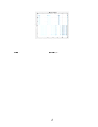
11. Answer:
Q1.41 MATLAB programs to generate the square- wave and the sawtooth wave se quences
of the type shown in Figures 1.1 and 1.2 are given below along with the sequences
generated by running these programs :
n = 0:30;
f = 0.1;
phase = 0; duty=60; A = 2.5;
arg = 2*pi*f*n + phase;
x = A*square(arg,duty);
clf;
stem(n,x);
axis([0 30 -3 3]); grid;
title('Onda cuadrada');
xlabel('n'); ylabel('Amplitud');
axis;
n = 0:30;
f = 0.1;
phase = 0;
duty=30;
A = 2.5;
arg = 2*pi*f*n + phase;
x = A*square(arg,duty);
clf;
stem(n,x);
axis([0 30 -3 3]); grid;
title('Onda cuadrada');
xlabel('n'); ylabel('Amplitud');
axis;
11

12. Date : Signature :
12