Downloaded 1,213 times


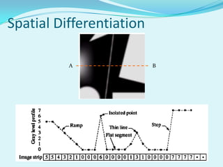
![Simple Neighbourhood Operations
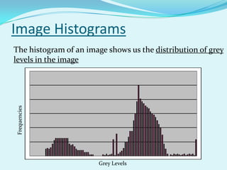
Some simple neighbourhood operations include:
Min:
Set the pixel value to the minimum in the neighbourhood
Max:
Set the pixel value to the maximum in the neighbourhood
Median:
The median value of a set of numbers is the midpoint value
in that set (e.g. from the set [1, 7, 15, 18, 24] 15 is the median).
Sometimes the median works better than the average](https://image.slidesharecdn.com/digitalimageprocessingimgsmoothning-120330085953-phpapp02/85/Digital-image-processing-img-smoothning-17-320.jpg)
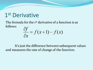
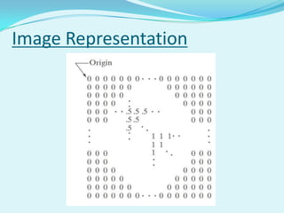
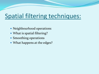
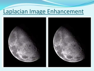
![The Laplacian (cont…)
So, the Laplacian can be given as follows:
2
f [ f ( x 1, y ) f ( x 1, y )
f ( x, y 1) f ( x, y 1)]
4 f ( x, y)
We can easily build a filter based on this
0 1 0
1 -4 1
0 1 0](https://image.slidesharecdn.com/digitalimageprocessingimgsmoothning-120330085953-phpapp02/85/Digital-image-processing-img-smoothning-28-320.jpg)
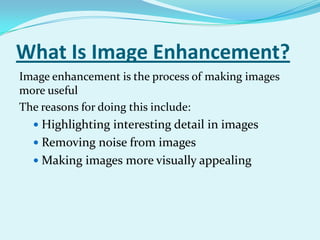
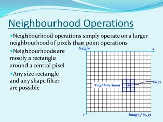
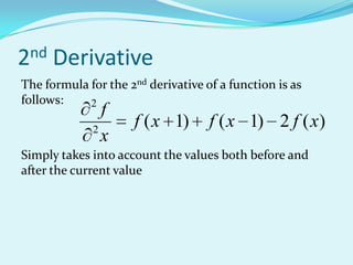
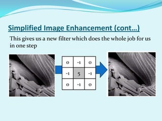
![Simplified Image Enhancement
The entire enhancement can be combined into a single
filtering operation
2
g ( x, y ) f ( x, y ) f
f ( x, y) [ f ( x 1, y) f ( x 1, y)
f ( x, y 1) f ( x, y 1)
4 f ( x, y)]
5 f ( x, y) f ( x 1, y) f ( x 1, y)
f ( x, y 1) f ( x, y 1)](https://image.slidesharecdn.com/digitalimageprocessingimgsmoothning-120330085953-phpapp02/85/Digital-image-processing-img-smoothning-33-320.jpg)
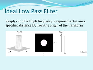
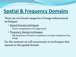
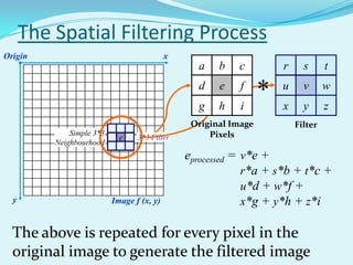
![Ideal Low Pass Filter (cont…)
The transfer function for the ideal low pass filter can be
given as:
1 if D(u, v) D0
H (u, v)
0 if D(u, v) D0
where D(u,v) is given as:
2 2 1/ 2
D(u, v) [(u M / 2) (v N / 2) ]](https://image.slidesharecdn.com/digitalimageprocessingimgsmoothning-120330085953-phpapp02/85/Digital-image-processing-img-smoothning-42-320.jpg)
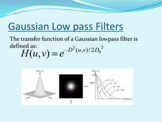
![Butterworth Low pass Filters
The transfer function of a Butterworth lowpass filter of
order n with cutoff frequency at distance D0 from the
origin is defined as:
1
H (u , v)
1 [ D(u , v) / D0 ]2 n](https://image.slidesharecdn.com/digitalimageprocessingimgsmoothning-120330085953-phpapp02/85/Digital-image-processing-img-smoothning-43-320.jpg)
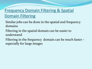
![Butterworth High Pass Filters
The Butterworth high pass filter is given as:
1
H (u , v) 2n
1 [ D0 / D(u , v)]
where n is the order and D0 is the cut off distance as
before](https://image.slidesharecdn.com/digitalimageprocessingimgsmoothning-120330085953-phpapp02/85/Digital-image-processing-img-smoothning-48-320.jpg)


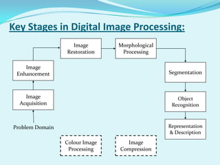
The document discusses image smoothing and sharpening techniques in digital image processing. It begins by defining what a digital image is and the goals of digital image processing. Then it discusses various applications of digital image processing like image enhancement, medical visualization, and human-computer interfaces. Key techniques covered include image smoothing using spatial filters to average pixel values in a neighborhood and image sharpening using spatial filters based on spatial differentiation to highlight edges. Examples of the Hubble space telescope and facial recognition are also mentioned.