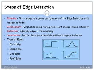
Download as PDF, PPTX
![Importance of Histograms Graph
24-09-2013©Kalyan Acharjya
27
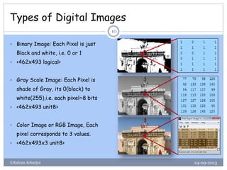
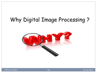
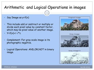
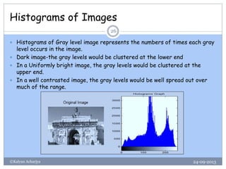
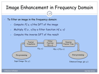
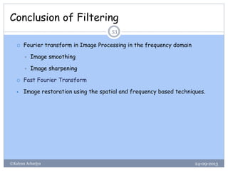
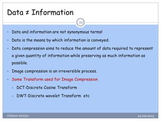
In Poorly Contrast image, enhance by spreading out of its histograms.
There are two ways-
Histograms stretching (contrast Stretching).
Histogram Equalization.
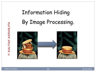
Histograms stretching:
• Poorly contrasted image in the range [a, b]
• Stretch the gray levels in the center of the range out by applying a
piecewise linear function.
• This function has the effect of stretching the gray levels [a, b] to
[c, d], where a<c and d>b](https://image.slidesharecdn.com/introductiontodigitalimageprocessing-140420015724-phpapp02/85/digital-image-processing-image-processing-27-320.jpg)
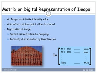
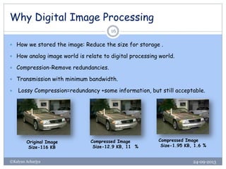
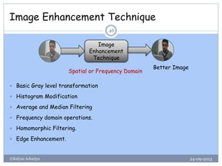
![Histograms stretching (Cont.)
24-09-2013©Kalyan Acharjya
28
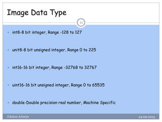
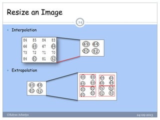
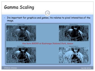
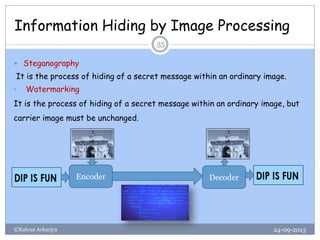
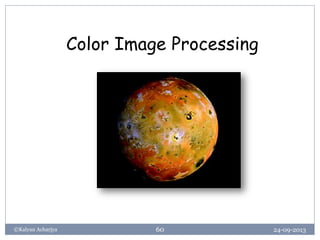
The linear function imadjust(I, [a, b],[c, d])
if Pixel value is less than c are all converted to c and pixel values greater
than d are all converted to d.
a b 1
c
d
1
Gamma<1 Gamma>1
Y= (
𝑥−𝑎
𝑏−𝑎
)^Gamma (d-c)+c](https://image.slidesharecdn.com/introductiontodigitalimageprocessing-140420015724-phpapp02/85/digital-image-processing-image-processing-28-320.jpg)
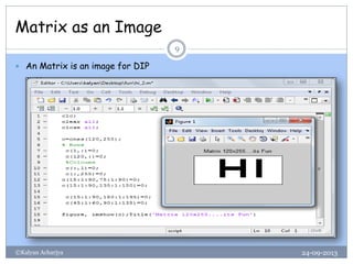
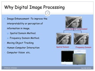
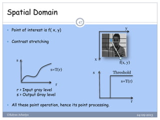
![Histograms Equalization
24-09-2013©Kalyan Acharjya
30
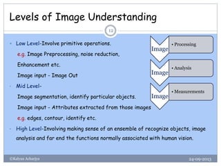
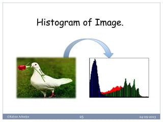
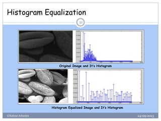
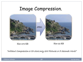
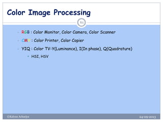
Histogram equalization is a technique for adjusting image intensities to
enhance contrast
• Histogram equalisation algorithm: Let be the
intensities of the image, and let be its normalised histogram
function. The intensity transformation function for histogram equalisation is
That is, we add the values of the normalised histogram function from 1
to k to find where the intensity will be mapped. Notice that the range
of the equalised image is the interval [0,1].
mkrk ,...,2,1,
)( krp
k
j
kk rprT
1
)()(
kr](https://image.slidesharecdn.com/introductiontodigitalimageprocessing-140420015724-phpapp02/85/digital-image-processing-image-processing-30-320.jpg)
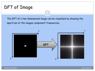
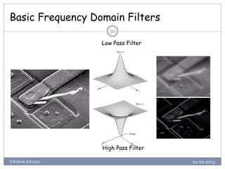
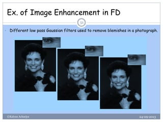
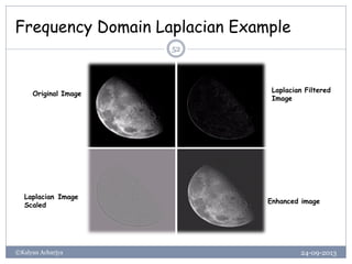

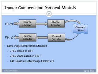


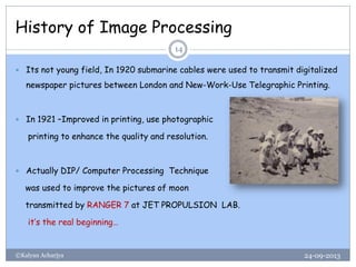
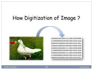
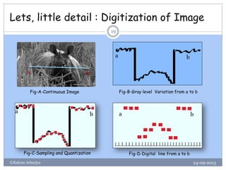
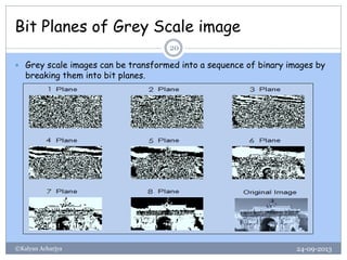
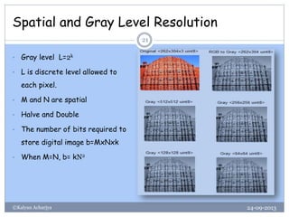
The document is a presentation by Kalyan Acharjya on digital image processing, covering its basic concepts, applications, and techniques such as image enhancement, noise extraction, and compression. It explains the definition of images, methods for digitization, and the importance of various processing techniques while also addressing topics like histogram manipulation and edge detection. The content serves educational purposes and includes historical context and technical details relevant to the field.