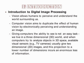
+IMAGE PROCESSING ANALYSIS,AND MACHINE
VISION MILAN SONKA VACLAV HLAVAC
ROGGER BOYYLE
+Rafael C. Ganzalez, Richard E. Woods, Digital
Image Processing, Second Edition, Y I.illl.
tti &*±, 2002.
+ John C. Russ, The Image Processing Handbook,
Fifth Edition, CRC Press, 2007.
1. Introduction
2. The digitized image and its properties
3. Data structures for image analysis
4. Image Pre-processing
5. Segmentation
6. Shape representation and description
7. Object recognition
8. Mathematical morphology
9. Texture
10. Image Understanding
+ Introduction to Digital Image Processing
- Vision allows humans to perceive and understand the
world surrounding us.
- Computer vision aims to duplicate the effect of human
vision by electronically perceiving and understanding
.
an image.
- Giving computers the ability to see is not an easy task -
we live in a three dimensional {3D) world, and when
computers try to analyze objects in 3D space, available
visual sensors (e.g., TV cameras) usually give two
dimensional (2D) images, and this projection to a
lower number of dimensions incurs an enormous loss
of information.
- In order to simplify the task of computer vision
understanding, two levels are usually distinguished;
low level image processing and high level image
understanding
- Low level methods usually use very little knowledge
about the content of images.
- High level processing is based on knowledge, goals,
and plans of how to achieve those goals. Artificial
intelligence (Al) methods are used in many cases.
High level computer vision tries to imitate human
cognition and the ability to make decisions according
to the information contained in the image.
+ Low level digital image processing
- Image Acquisition
x An image is captured by a sensor {such as a TV camera) and
digitized;
- Preprocessing
x computer suppresses noise {image pre-processing) and maybe
enhances some object features which are relevant to
understanding the image. Edge extraction is an example of
processing carried out at this stage.
- Image segmentation
x computer tries to separate objects from the image background.
- Object description and classification
x Object description and classification in a totally segmented image
is also understood as part of low level image processing.
+ Overview:
- 2.1 Basic Concepts
x Image functions
x The Dirac distribution and convolution
x The Fourier transform
x Images as a stochastic process
- 2.2 Image digitization
x Sampling
x Quantization
x Color images
- 2.3 Digital image properties
x Metric and topological properties of digital images
x Histograms
x Visual perception of the image
x Image quality
x Noise in images
+ Fundamental concepts and mathematical tools are introduced in this
chapter which will be used throughout the course.
+ A signal is a function depending on some variable with
physical meaning.
+ Signals can be
- one-dimensional (e.g., dependent on time),
- two-dimensional (e.g., images dependent on two co-ordinates
in a plane),
- three-dimensional (e.g., describing an object in space),
- or higher-dimensional.
+ A scalar function may be sufficient to describe a
monochromatici mage, while vector functions are used in
image processing to represent , for example, color images
consisting of three component colors.
+ Computerized image processing uses digital image functions
which are usually represented by matrices, so co-ordinates
are integer numbers.
+ The customary orientation of co-ordinates in an image is in
the normal Cartesian fashion (horizontal x axis, vertical y
axis), although the (row, column) orientation used in
matrices is also quite often used in digital image processing.
 + The range of image function values is also limited; by
convention, in monochromatic images the lowest value
corresponds to black and the highest to white.
 + Brightness values bounded by these limits are
gray levels.

In computer vision, an image is often represented as a
function that maps a set of coordinates to pixel values. This
function is typically referred to as the image function or
image signal.
 The image function takes these coordinates as input and
returns the corresponding pixel value. The pixel value
represents the intensity or color of the pixel at that location.
For grayscale images, the pixel value is usually a single value
ranging from 0 to 255, where 0 represents black and 255
represents white. For color images, the pixel value is typically
a combination of three values representing the intensities of
red, green, and blue channels.
 By treating an image as a function, we can perform various
operations on it using mathematical techniques. For
example, we can apply filters or transformations to the image
function to enhance certain features or extract useful
information.
+ The discretization of images from a
continuous domain can be achieved by
convolution with Dirac functions.
The ideal impulse in the image plane is defined
using the Dirac distribution delta( x,y)dx dy=1
delta(x,y)=0for all x,ynot=0.
The convolution expresses a linear filtering
process using filter h;linear filtering is often
used in local image preprocessing and image
restoration.
+ We will discuss this question in the next course.
+ Images f(x,y) can be treated as deterministic
functions or as realizations of stochastic
processes.
+ Mathematical tools used in image description
have roots in linear system theory, integral
transformations, discrete mathematics and
the theory of stochastic processes.
+ An image captured by a sensor is expressed as a
continuous function f(x,y) of two co-ordinates in the
plane.
+ Image digitization means that the function f(x,y) is
sampled( t¥) into a matrix with M rows and N
columns.
+ The image quantitation(:i:it) assigns to each
continuous sample an integer value.
+ The continuous range of the image function f(x,y) is
split into K intervals.
+ The finer the sampling (i.e., the larger M and N) and
quantitation (the larger K) the better the
approximation of the continuous image function
f(x,y).
+ Two questions should be answered in
connection with image function sampling:
- First, the sampling period should be determined -
the distance between two neighboring sampling
points in the image
- Second, the geometric arrangement of sampling
points (sampling g r i d * ¥tfffi{a) should be set.
+ A continuous image function
f(x,y) can be sampled using a
discrete grid of sampling
points in the plane.
+ The image is sampled at points x = j x, y = k y
+ Two neighboring sampling points are separated
by distance x along the x axis and y along the
y axis. Distances x and y are called the
sampling interval(*t¥f8] i;) and the matrix of
samples constitutes the discrete image.
+ The ideal sampling s(x,y) in the regular grid can be
represented using a collection of Dirac distributions
M
r N
s(x,y) - ! l ( x JtjM,y �)
j C k •
+ The sampled image is the product of the continuous
image f(x,y) and the sampling function s(x,y)
(f s)(x, y)
fs(x, y) -
M J,,T
LL f ( x , y ) 6 ( x - j x , y - k y )
-
.i=l k=l
M J,,T
(2.32)
- f(x,y) LL 6 ( x - j x , y - k y )
; i =l k =l
+ The collection of Dirac distributions in equation
2.32 can be regarded as periodic with period x, y
and expanded into a Fourier series (assuming that
the sampling grid covers the whole plane (infinite
limits)) . (Eq. 2.33)
oc oc
E E
,i=-oc k=-oc
oc oc
6 ( x - j x , y - k y ) = E E U m i i e
2
r i ( + ) (2.33)
m=-oc n=-oc
+ where the coefficients of the Fourier expansion
can be calculated as given in Eq. 2.34
(2.34)
+ Noting that only the term for j=O and k=O in the
sum is nonzero in the range of integration, the
coefficients are in Eq. 2.35
(2.35)
+ Noting that the integral in equation 2.35 is
uniformly equal to one the coefficients can be
expressed as given in Eq. 2.36 and 2.32 can be
rewritten as Eq. 2.37.
+ In frequency domain then Eq. 2.38.
(2.36)
l oc oc
/( "' "' 2 r i ( + . ! ! l l . . )
fs (x,y) = ·x,y) -- L..J L..J e &s; .&a,
� X �Y -m= - oc -n=-oc
oc oc
1
Fs(u.,u) = x ,E
j
E F ( u . - x ' v - )
Y . 1 = - o c k = - o c
k
Y
(2.37)
(2.38)
+ Thus the Fourier transform of the sampled image is the
sum of periodically repeated Fourier transforms F(u,v)
of the image.
+ Periodic repetition of the Fourier transform result F(u,v)
may under certain conditions cause distortion of the
image which is called aliasing(& ); this happens
when individual digitized components F(u,v) overlap(
I).
function f(x,y) has a
band l i m i t e d ( I * M) s p e c t r u m ( ii) ... its
Fourier transform F(u,v)=O outside a certain interval
of frequencies Iu I > U; Iv I > V.
+ As you know from general sampling theory,
overlapping of the periodically repeated results of
the Fourier transform F(u,v) of an image with band
limited spectrum can be prevented if the sampling
interval is chosen according to Eq. 2.39
(2.39)
+ This is the Shannon sampling theorem that has a
simple physical interpretation in image analysis: The
sampling interval should be chosen in size such that
it is less than or equal to half of the smallest
interesting detail in the image.
+ The sampling function is not the Dirac distribution in
real digitizers -- narrow impulses with limited
amplitude( ,&;qJ;fl ) are used instead.
+ As a result, in real image digitizers a sampling
interval about ten times smaller than that indicated
by the Shannon sampling theorem is used - because
the algorithms for image reconstruction use only a
step function( fi' l2EJi9:).
+ Practical examples of digitization using a flatbed scanner and TV
cameras help to understand the reality of sampling.
Original image
half
lOx
twice
+ A continuous image is digitized at sampling points{
- ; - i ' ' 2S'
*rr=FI
   ) •
+ These sampling points are ordered in the plane and
their geometric relation is called the grid(lltffi).
+ Grids used in practice are mainly square or
hexagonal {Figure 2.4).
(a) (b)
Figure 2.4 (a) Squat-e 9rid, (b) heza9on.ai 9rid.
point in the grid corresponds
to one picture element
(pixelit•) in the digital image.
+ The set of pixels together covers the entire image.
+ Pixels captured by a real digitization device have
finite sizes.
+ The pixel is a unit which is not further divisible,
sometimes pixels are also called points.
digital value in image
processing.
+ The transition between continuous values of
the image function {brightness) and its digital
equivalent is called quantitation(.il:).
+ The number of quantitation levels should be
high enough for human perception of fine
shading details in the image.
+ Most digital image
processing devices use
quantitation into k equal intervals( faJ 1¥.1).
+ If b bits are used ... the number of brightness
levels is k=2b.
+ Eight bits per pixel are commonly used,
specialized measuring devices use twelve and
more bits per pixel.
+ Metric and topological( ! ) properties of
digital images
+ Histograms(il/JIII)
+ Visual perception of the image
+ Image quality
+ Noise in images
straightforward analogy(
f
l
1t:.Ul)) in the domain of
digital images.
+ Distance is an important example.
+ The distance between two pixels in a digital
image is a significant quantitative measure.
+ The distance between points with co-ordinates
(i,j) and (h,k) may be defined in several
different ways;
- the Euclidean distance is defined by Eq. 2.42
DE((i,j),(h.,k))=( i - h.)2
+(j - k)2
(2.42)
- city block distance ... Eq. 2.43
D4((i,j),(h.,k))==Ii - h
.I +I j - kI (2.43)
- chessboard distance Eq. 2.44
D B ( ( i , j ) , ( h . , k ) ) =
=max{Ii - h. I, I j- k I} (2.44)
+ Pixel adjacency( IHl•ti) is another important
concept in digital images.
+ 4-neighborhood
+ 8-neighborhood (Fig. 2.6)
Figure 2.0 Piul nei9hho,urhoods.
+ It will become necessary to consi er important
sets consisting of several adjacent pixels -
regions(l&Jil).
I I
■
■ ■ ■ ■ ■
■ ■ ■ ■
■ ■ ■ ■
■ ■ ■ ■
■ ■ ■
■ ■
■ ■ ■ ■ ■ ■
■ ■ ■ ■ ■ ■ ■
■ ■ ■
■ ■ ■
■ ■
■ ■
■ ■
■ ■
+ Region is a contiguous(ii®8{]) set.
+ Contiguity paradoxes(1$i.t) of the square grid
... Fig. 2.7, 2.8
I
I
I
Figure Z.7 Di9ital line. Figure Z.8 Olosed curtte paradcn.
objects using 4-neighborhood
and background using 8-
neighborhood (or vice versa).
+ A hexagonal grid solves many problems of the
square grids ... any point in the hexagonal raster(
7CM)has the same distance to all its six
neighbors.
+ Border(jn ) R is the set of pixels within the region
that have one or more neighbors outside R ... inner
borders, outer borders exist.
+ E d g e ( j n ) is a local property of a
pixel and its immediate ( I J l )
neighborhood --it is a vector(
: I : ) given by a magnitude and direction.
+ The edge direction is perpendicular to the gradient
(*tN)direction which points in the direction of
image function growth.
+ Border and edge ... the border is a global concept
related to a region, while edge expresses local
properties of an image function.
+ Crack(llti) edges ... four crack edges are
attached to each pixel, which are defined by its
relation to its 4-neighbors. The direction of the
crack edge is that of increasing brightness, and is
a multiple{itiO of 90 degrees, while its
magnitude is the absolute difference( )
between the brightness of the relevant pair of
pixels. (Fig. 2.9)
F i g u r e 2.9 Oro.ck edges.
+ Topological properties of
images are invariant
to rubber sheet transformations(.Stiii ).
+ Stretching(i$Jm) does not change contiguity of
the object parts and does not change the
number of holes(fL) in regions.
+ One such image property is the Euler--Poincare
characteristic defined as the difference( )
between the number of regions and the
number of holes in them.
+ Convex hull(8'2!) is used to describe topological
properties of objects.
+ The convex hull is the smallest region which
contains the object, such that any two points of
the region can be connected by a straight line, all
points of which belong to the region.
Figure 2.10 Description min9 topo/09ioo/ oomponents: (a) An 'R1
object,
(/J) its cont1e:z: hull, (c) ,akes and bays.
+ Brightness histogram provides the frequency
of the brightness value z in the image.
1000
1
800 r
soo r
i
700
i
600
i
soo r
400
300 L
i
!
200
I
1
0
0
0 .............
0 32
G
C
:
c:,
u
cr
.
c
_
u
LL
64 86 128 160 192 224
Intensity
Figure 2.11 A brightness histogram.
1. Assign zero values to all
elements of the array h.
2. For all pixels (x,y) of the image f, increment
h(f(x,y)) by one.
int h{256}={0};
for(i=O; i<M;i++)
for(j=O; j<N;j++)
h[f[i][j]]++;
+ Histograms may have many local maxima(*&
11)...
+ histogram smoothing( /JOOIJZ )
hf(z) = l t h1(z +i),
2K +1 i=-K
(2.45)
+ Images are often degraded( it) by random
noi•
se.
+ Noise can occur during image capture,
transmission or processing, and may be
dependent on or independent of image
content.
+ Noise is usually described by its probabilistic
characteristics.
- White noise - constant power spectrum {its intensity
does not decrease with increasing frequency); very
crude approximation of image noise;
- Gaussian noise is a very good approximation of noise
that occurs in many practical cases;
- probability density of the random variable is given by
the Gaussian curve;
- 1D Gaussian noise - µ is the mean and is the standard
deviation of the random variable.
1
p(x) = - - e 2 a 2
-(.x-µ.)2
a � '
independent of the image
signal occurs.
+ Noise may be
- additive, noise and image signal g are independent
f(x, y)= g(x, y) + v(x,y),
- multiplicative, noise is a function of signal magnitude
f = g + vg = g(l + v) gv
- impulse noise (saturatedt§fD = salt and pepper noise)
Original image Noise degraded image
+ SignaI-to-noise ratio(SNR)
- Computing the total square value of the noise
contribution E • yw2 , , yJ
41t,y,
- The total square value of the observed signal
F • ! 12,,y,
- SNR
chAPTER1CV.pptx is abouter computer vision in artificial intelligence

chAPTER1CV.pptx is abouter computer vision in artificial intelligence

  • 14.
    +IMAGE PROCESSING ANALYSIS,ANDMACHINE VISION MILAN SONKA VACLAV HLAVAC ROGGER BOYYLE +Rafael C. Ganzalez, Richard E. Woods, Digital Image Processing, Second Edition, Y I.illl. tti &*±, 2002. + John C. Russ, The Image Processing Handbook, Fifth Edition, CRC Press, 2007.
  • 16.
    1. Introduction 2. Thedigitized image and its properties 3. Data structures for image analysis 4. Image Pre-processing 5. Segmentation 6. Shape representation and description 7. Object recognition 8. Mathematical morphology 9. Texture 10. Image Understanding
  • 17.
    + Introduction toDigital Image Processing - Vision allows humans to perceive and understand the world surrounding us. - Computer vision aims to duplicate the effect of human vision by electronically perceiving and understanding . an image. - Giving computers the ability to see is not an easy task - we live in a three dimensional {3D) world, and when computers try to analyze objects in 3D space, available visual sensors (e.g., TV cameras) usually give two dimensional (2D) images, and this projection to a lower number of dimensions incurs an enormous loss of information.
  • 18.
    - In orderto simplify the task of computer vision understanding, two levels are usually distinguished; low level image processing and high level image understanding - Low level methods usually use very little knowledge about the content of images. - High level processing is based on knowledge, goals, and plans of how to achieve those goals. Artificial intelligence (Al) methods are used in many cases. High level computer vision tries to imitate human cognition and the ability to make decisions according to the information contained in the image.
  • 19.
    + Low leveldigital image processing - Image Acquisition x An image is captured by a sensor {such as a TV camera) and digitized; - Preprocessing x computer suppresses noise {image pre-processing) and maybe enhances some object features which are relevant to understanding the image. Edge extraction is an example of processing carried out at this stage. - Image segmentation x computer tries to separate objects from the image background. - Object description and classification x Object description and classification in a totally segmented image is also understood as part of low level image processing.
  • 22.
    + Overview: - 2.1Basic Concepts x Image functions x The Dirac distribution and convolution x The Fourier transform x Images as a stochastic process - 2.2 Image digitization x Sampling x Quantization x Color images - 2.3 Digital image properties x Metric and topological properties of digital images x Histograms x Visual perception of the image x Image quality x Noise in images
  • 23.
    + Fundamental conceptsand mathematical tools are introduced in this chapter which will be used throughout the course. + A signal is a function depending on some variable with physical meaning. + Signals can be - one-dimensional (e.g., dependent on time), - two-dimensional (e.g., images dependent on two co-ordinates in a plane), - three-dimensional (e.g., describing an object in space), - or higher-dimensional. + A scalar function may be sufficient to describe a monochromatici mage, while vector functions are used in image processing to represent , for example, color images consisting of three component colors.
  • 24.
    + Computerized imageprocessing uses digital image functions which are usually represented by matrices, so co-ordinates are integer numbers. + The customary orientation of co-ordinates in an image is in the normal Cartesian fashion (horizontal x axis, vertical y axis), although the (row, column) orientation used in matrices is also quite often used in digital image processing.  + The range of image function values is also limited; by convention, in monochromatic images the lowest value corresponds to black and the highest to white.  + Brightness values bounded by these limits are gray levels.
  • 28.
     In computer vision,an image is often represented as a function that maps a set of coordinates to pixel values. This function is typically referred to as the image function or image signal.  The image function takes these coordinates as input and returns the corresponding pixel value. The pixel value represents the intensity or color of the pixel at that location. For grayscale images, the pixel value is usually a single value ranging from 0 to 255, where 0 represents black and 255 represents white. For color images, the pixel value is typically a combination of three values representing the intensities of red, green, and blue channels.  By treating an image as a function, we can perform various operations on it using mathematical techniques. For example, we can apply filters or transformations to the image function to enhance certain features or extract useful information.
  • 29.
    + The discretizationof images from a continuous domain can be achieved by convolution with Dirac functions. The ideal impulse in the image plane is defined using the Dirac distribution delta( x,y)dx dy=1 delta(x,y)=0for all x,ynot=0. The convolution expresses a linear filtering process using filter h;linear filtering is often used in local image preprocessing and image restoration.
  • 30.
    + We willdiscuss this question in the next course.
  • 31.
    + Images f(x,y)can be treated as deterministic functions or as realizations of stochastic processes. + Mathematical tools used in image description have roots in linear system theory, integral transformations, discrete mathematics and the theory of stochastic processes.
  • 32.
    + An imagecaptured by a sensor is expressed as a continuous function f(x,y) of two co-ordinates in the plane. + Image digitization means that the function f(x,y) is sampled( t¥) into a matrix with M rows and N columns. + The image quantitation(:i:it) assigns to each continuous sample an integer value. + The continuous range of the image function f(x,y) is split into K intervals.
  • 33.
    + The finerthe sampling (i.e., the larger M and N) and quantitation (the larger K) the better the approximation of the continuous image function f(x,y). + Two questions should be answered in connection with image function sampling: - First, the sampling period should be determined - the distance between two neighboring sampling points in the image - Second, the geometric arrangement of sampling points (sampling g r i d * ¥tfffi{a) should be set.
  • 34.
    + A continuousimage function f(x,y) can be sampled using a discrete grid of sampling points in the plane. + The image is sampled at points x = j x, y = k y + Two neighboring sampling points are separated by distance x along the x axis and y along the y axis. Distances x and y are called the sampling interval(*t¥f8] i;) and the matrix of samples constitutes the discrete image.
  • 35.
    + The idealsampling s(x,y) in the regular grid can be represented using a collection of Dirac distributions M r N s(x,y) - ! l ( x JtjM,y �) j C k • + The sampled image is the product of the continuous image f(x,y) and the sampling function s(x,y) (f s)(x, y) fs(x, y) - M J,,T LL f ( x , y ) 6 ( x - j x , y - k y ) - .i=l k=l M J,,T (2.32) - f(x,y) LL 6 ( x - j x , y - k y ) ; i =l k =l
  • 36.
    + The collectionof Dirac distributions in equation 2.32 can be regarded as periodic with period x, y and expanded into a Fourier series (assuming that the sampling grid covers the whole plane (infinite limits)) . (Eq. 2.33) oc oc E E ,i=-oc k=-oc oc oc 6 ( x - j x , y - k y ) = E E U m i i e 2 r i ( + ) (2.33) m=-oc n=-oc + where the coefficients of the Fourier expansion can be calculated as given in Eq. 2.34 (2.34)
  • 37.
    + Noting thatonly the term for j=O and k=O in the sum is nonzero in the range of integration, the coefficients are in Eq. 2.35 (2.35) + Noting that the integral in equation 2.35 is uniformly equal to one the coefficients can be expressed as given in Eq. 2.36 and 2.32 can be rewritten as Eq. 2.37. + In frequency domain then Eq. 2.38.
  • 38.
    (2.36) l oc oc /("' "' 2 r i ( + . ! ! l l . . ) fs (x,y) = ·x,y) -- L..J L..J e &s; .&a, � X �Y -m= - oc -n=-oc oc oc 1 Fs(u.,u) = x ,E j E F ( u . - x ' v - ) Y . 1 = - o c k = - o c k Y (2.37) (2.38) + Thus the Fourier transform of the sampled image is the sum of periodically repeated Fourier transforms F(u,v) of the image. + Periodic repetition of the Fourier transform result F(u,v) may under certain conditions cause distortion of the image which is called aliasing(& ); this happens when individual digitized components F(u,v) overlap( I).
  • 39.
    function f(x,y) hasa band l i m i t e d ( I * M) s p e c t r u m ( ii) ... its Fourier transform F(u,v)=O outside a certain interval of frequencies Iu I > U; Iv I > V. + As you know from general sampling theory, overlapping of the periodically repeated results of the Fourier transform F(u,v) of an image with band limited spectrum can be prevented if the sampling interval is chosen according to Eq. 2.39 (2.39)
  • 40.
    + This isthe Shannon sampling theorem that has a simple physical interpretation in image analysis: The sampling interval should be chosen in size such that it is less than or equal to half of the smallest interesting detail in the image. + The sampling function is not the Dirac distribution in real digitizers -- narrow impulses with limited amplitude( ,&;qJ;fl ) are used instead. + As a result, in real image digitizers a sampling interval about ten times smaller than that indicated by the Shannon sampling theorem is used - because the algorithms for image reconstruction use only a step function( fi' l2EJi9:).
  • 41.
    + Practical examplesof digitization using a flatbed scanner and TV cameras help to understand the reality of sampling. Original image half lOx twice
  • 42.
    + A continuousimage is digitized at sampling points{ - ; - i ' ' 2S' *rr=FI ) • + These sampling points are ordered in the plane and their geometric relation is called the grid(lltffi). + Grids used in practice are mainly square or hexagonal {Figure 2.4). (a) (b) Figure 2.4 (a) Squat-e 9rid, (b) heza9on.ai 9rid.
  • 43.
    point in thegrid corresponds to one picture element (pixelit•) in the digital image. + The set of pixels together covers the entire image. + Pixels captured by a real digitization device have finite sizes. + The pixel is a unit which is not further divisible, sometimes pixels are also called points.
  • 44.
    digital value inimage processing. + The transition between continuous values of the image function {brightness) and its digital equivalent is called quantitation(.il:). + The number of quantitation levels should be high enough for human perception of fine shading details in the image.
  • 45.
    + Most digitalimage processing devices use quantitation into k equal intervals( faJ 1¥.1). + If b bits are used ... the number of brightness levels is k=2b. + Eight bits per pixel are commonly used, specialized measuring devices use twelve and more bits per pixel.
  • 46.
    + Metric andtopological( ! ) properties of digital images + Histograms(il/JIII) + Visual perception of the image + Image quality + Noise in images
  • 47.
    straightforward analogy( f l 1t:.Ul)) inthe domain of digital images.
  • 48.
    + Distance isan important example. + The distance between two pixels in a digital image is a significant quantitative measure. + The distance between points with co-ordinates (i,j) and (h,k) may be defined in several different ways;
  • 49.
    - the Euclideandistance is defined by Eq. 2.42 DE((i,j),(h.,k))=( i - h.)2 +(j - k)2 (2.42) - city block distance ... Eq. 2.43 D4((i,j),(h.,k))==Ii - h .I +I j - kI (2.43) - chessboard distance Eq. 2.44 D B ( ( i , j ) , ( h . , k ) ) = =max{Ii - h. I, I j- k I} (2.44)
  • 50.
    + Pixel adjacency(IHl•ti) is another important concept in digital images. + 4-neighborhood + 8-neighborhood (Fig. 2.6) Figure 2.0 Piul nei9hho,urhoods. + It will become necessary to consi er important sets consisting of several adjacent pixels - regions(l&Jil).
  • 51.
    I I ■ ■ ■■ ■ ■ ■ ■ ■ ■ ■ ■ ■ ■ ■ ■ ■ ■ ■ ■ ■ ■ ■ ■ ■ ■ ■ ■ ■ ■ ■ ■ ■ ■ ■ ■ ■ ■ ■ ■ ■ ■ ■ ■ ■ ■ ■ ■ ■ ■ + Region is a contiguous(ii®8{]) set. + Contiguity paradoxes(1$i.t) of the square grid ... Fig. 2.7, 2.8 I I I Figure Z.7 Di9ital line. Figure Z.8 Olosed curtte paradcn.
  • 52.
    objects using 4-neighborhood andbackground using 8- neighborhood (or vice versa). + A hexagonal grid solves many problems of the square grids ... any point in the hexagonal raster( 7CM)has the same distance to all its six neighbors.
  • 53.
    + Border(jn )R is the set of pixels within the region that have one or more neighbors outside R ... inner borders, outer borders exist. + E d g e ( j n ) is a local property of a pixel and its immediate ( I J l ) neighborhood --it is a vector( : I : ) given by a magnitude and direction. + The edge direction is perpendicular to the gradient (*tN)direction which points in the direction of image function growth. + Border and edge ... the border is a global concept related to a region, while edge expresses local properties of an image function.
  • 54.
    + Crack(llti) edges... four crack edges are attached to each pixel, which are defined by its relation to its 4-neighbors. The direction of the crack edge is that of increasing brightness, and is a multiple{itiO of 90 degrees, while its magnitude is the absolute difference( ) between the brightness of the relevant pair of pixels. (Fig. 2.9) F i g u r e 2.9 Oro.ck edges.
  • 55.
    + Topological propertiesof images are invariant to rubber sheet transformations(.Stiii ). + Stretching(i$Jm) does not change contiguity of the object parts and does not change the number of holes(fL) in regions. + One such image property is the Euler--Poincare characteristic defined as the difference( ) between the number of regions and the number of holes in them.
  • 56.
    + Convex hull(8'2!)is used to describe topological properties of objects. + The convex hull is the smallest region which contains the object, such that any two points of the region can be connected by a straight line, all points of which belong to the region. Figure 2.10 Description min9 topo/09ioo/ oomponents: (a) An 'R1 object, (/J) its cont1e:z: hull, (c) ,akes and bays.
  • 57.
    + Brightness histogramprovides the frequency of the brightness value z in the image. 1000 1 800 r soo r i 700 i 600 i soo r 400 300 L i ! 200 I 1 0 0 0 ............. 0 32 G C : c:, u cr . c _ u LL 64 86 128 160 192 224 Intensity Figure 2.11 A brightness histogram.
  • 58.
    1. Assign zerovalues to all elements of the array h. 2. For all pixels (x,y) of the image f, increment h(f(x,y)) by one. int h{256}={0}; for(i=O; i<M;i++) for(j=O; j<N;j++) h[f[i][j]]++;
  • 59.
    + Histograms mayhave many local maxima(*& 11)... + histogram smoothing( /JOOIJZ ) hf(z) = l t h1(z +i), 2K +1 i=-K (2.45)
  • 60.
    + Images areoften degraded( it) by random noi• se. + Noise can occur during image capture, transmission or processing, and may be dependent on or independent of image content.
  • 61.
    + Noise isusually described by its probabilistic characteristics. - White noise - constant power spectrum {its intensity does not decrease with increasing frequency); very crude approximation of image noise; - Gaussian noise is a very good approximation of noise that occurs in many practical cases; - probability density of the random variable is given by the Gaussian curve; - 1D Gaussian noise - µ is the mean and is the standard deviation of the random variable. 1 p(x) = - - e 2 a 2 -(.x-µ.)2 a � '
  • 62.
    independent of theimage signal occurs. + Noise may be - additive, noise and image signal g are independent f(x, y)= g(x, y) + v(x,y), - multiplicative, noise is a function of signal magnitude f = g + vg = g(l + v) gv - impulse noise (saturatedt§fD = salt and pepper noise)
  • 63.
    Original image Noisedegraded image
  • 64.
    + SignaI-to-noise ratio(SNR) -Computing the total square value of the noise contribution E • yw2 , , yJ 41t,y, - The total square value of the observed signal F • ! 12,,y, - SNR