


![Introduction Basis functions Hartree–Fock Density functional theory Time–dependent DFT End
Bases in function spaces
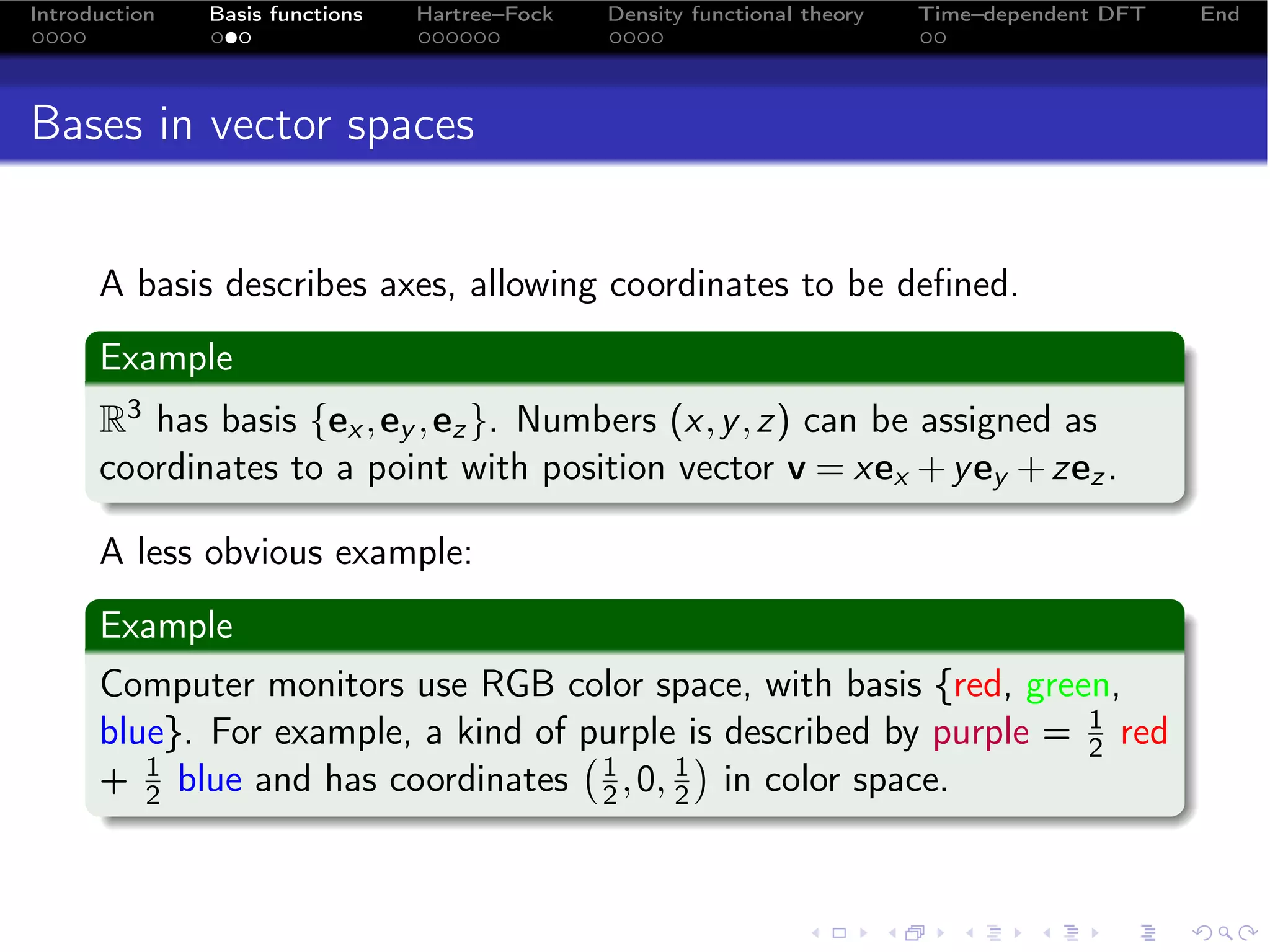
Basis functions describe “axes” in function space. If you have a
collection of mutually orthogonal, real functions φ1 (x) , . . . , φn (x)
that span the entire space of functions, then
f (x) = ∑ ci φi (x) (7)
i
whose coefficients are given by projections onto the basis
N f (x) φi (x) dx
´
ci = R´ 2
(8)
RN φi (x) dx
Then the function f has “coordinates” (c1 , c2 , . . . ) in the basis
spanning the function space.
Example
Functions over [−π, π] have Fourier series expansions, whose basis
functions are 1, sin x, cos 2x, sin 3x, cos 4x, . . .](https://image.slidesharecdn.com/efrc-lunch-100311234948-phpapp01/75/A-brief-introduction-to-Hartree-Fock-and-TDDFT-11-2048.jpg)
![Introduction Basis functions Hartree–Fock Density functional theory Time–dependent DFT End
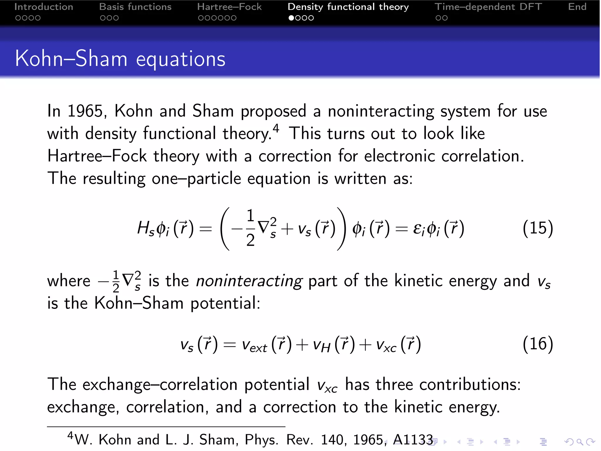
Kohn–Sham is a density functional theory
The Kohn–Sham equation is equivalent to finding the density ρ
that minimizes the energy functional
ˆ
E [ρ] = vext (r ) ρ (r ) d + Ts [ρ] + VH [ρ] + Exc [ρ]
r (17)
R3
1 N
ˆ
Ts [ρ] = − ∑ φi (r ) ∇2 φi (r ) d
r (18)
2 i=1 R3
1 ρ (r ) ρ (r )
ˆ
VH [ρ] = + d d
r r (19)
2 R6 |r −
r |
where the density is constructed from
N
ρ (r ) =
∑ |φi ( )|2 = ∑
r Ci µ Ciν χµ (r ) χν (r )
(20)
i=1 µνi](https://image.slidesharecdn.com/efrc-lunch-100311234948-phpapp01/75/A-brief-introduction-to-Hartree-Fock-and-TDDFT-19-2048.jpg)
![Introduction Basis functions Hartree–Fock Density functional theory Time–dependent DFT End
Density functionals
The form of the exchange–correlation functional Exc is unknown.
There are many, many approximations to it:
“Jacob’s Ladder” of approximations to Exc [ρ]:5
1 Exc [ρ] LDA X α, LDA,...
2 Exc [ρ, ∇ρ] GGA BLYP, PBE, PW91...
3 Exc [ρ, ∇ρ, τ] meta–GGA VSXC, TPSS, ...
4 Exc [ρ, ∇ρ, τ, {φ }o ] hybrids 6 ,... B3LYP, PBE0,...
5 Exc [ρ, ∇ρ, τ, {φ }] fully nonlocal -
LDA, local density approximation; GGA, generalized gradient
approximation; τ, kinetic energy density; {φ }o , occupied
orbitals; {φ }, all orbitals.
Green function expansions for Exc : GW, Görling–Levy PT,...
Approximations to kinetic energy: Thomas–Fermi, von
Wiezsäcker,...
5 M. Casida, http://bit.ly/casidadft
6 Hybrid functionals mix in Hartree–Fock exchange.](https://image.slidesharecdn.com/efrc-lunch-100311234948-phpapp01/75/A-brief-introduction-to-Hartree-Fock-and-TDDFT-20-2048.jpg)

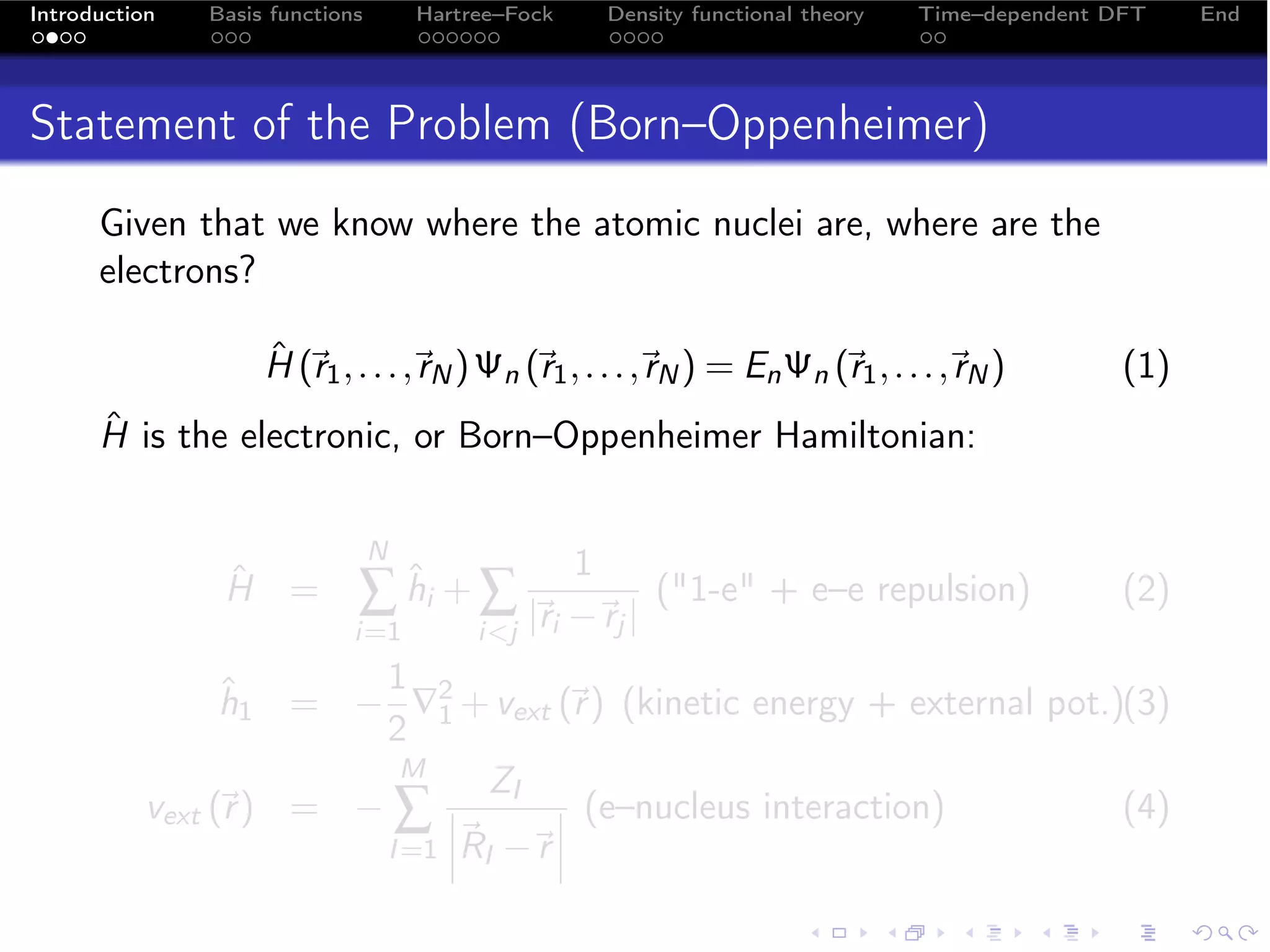
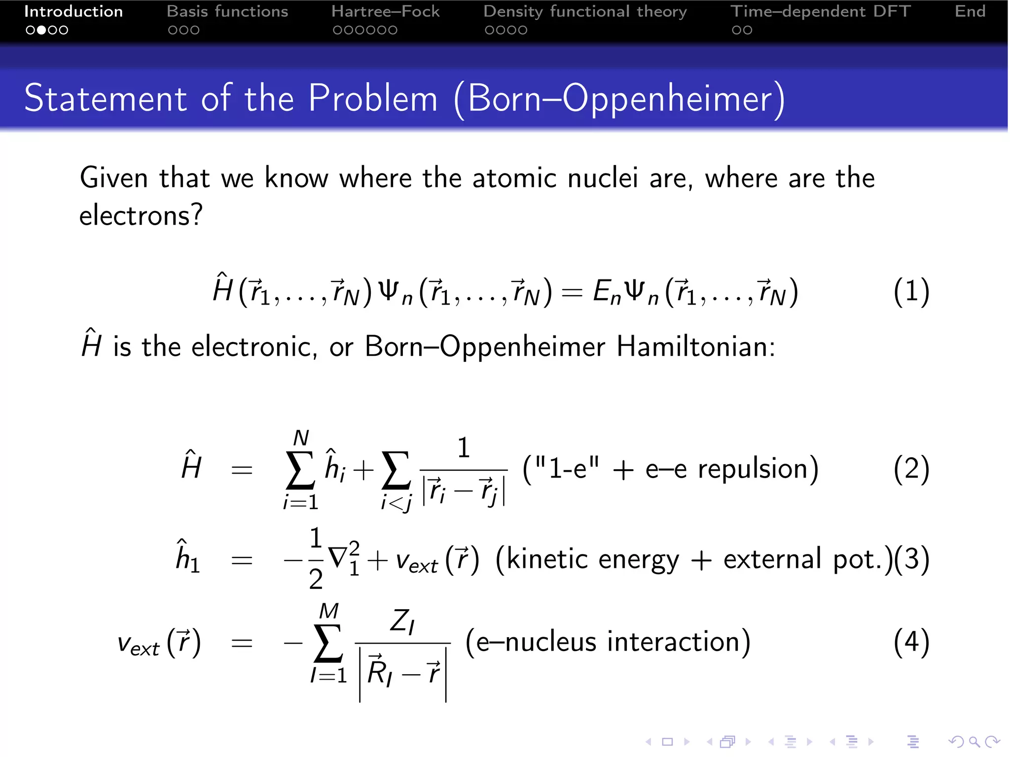
The document provides an overview of time-dependent density functional theory (TDDFT) for computing molecular excited states. It begins with an introduction to the Born-Oppenheimer approximation and variational principle. It then discusses the Hartree-Fock and Kohn-Sham equations as self-consistent field methods for calculating ground states, and linear response theory for calculating excited states within TDDFT. The contents section outlines the topics to be covered, including basis functions, Hartree-Fock theory, density functional theory, and time-dependent DFT.