Downloaded 437 times


![Matlab Verification
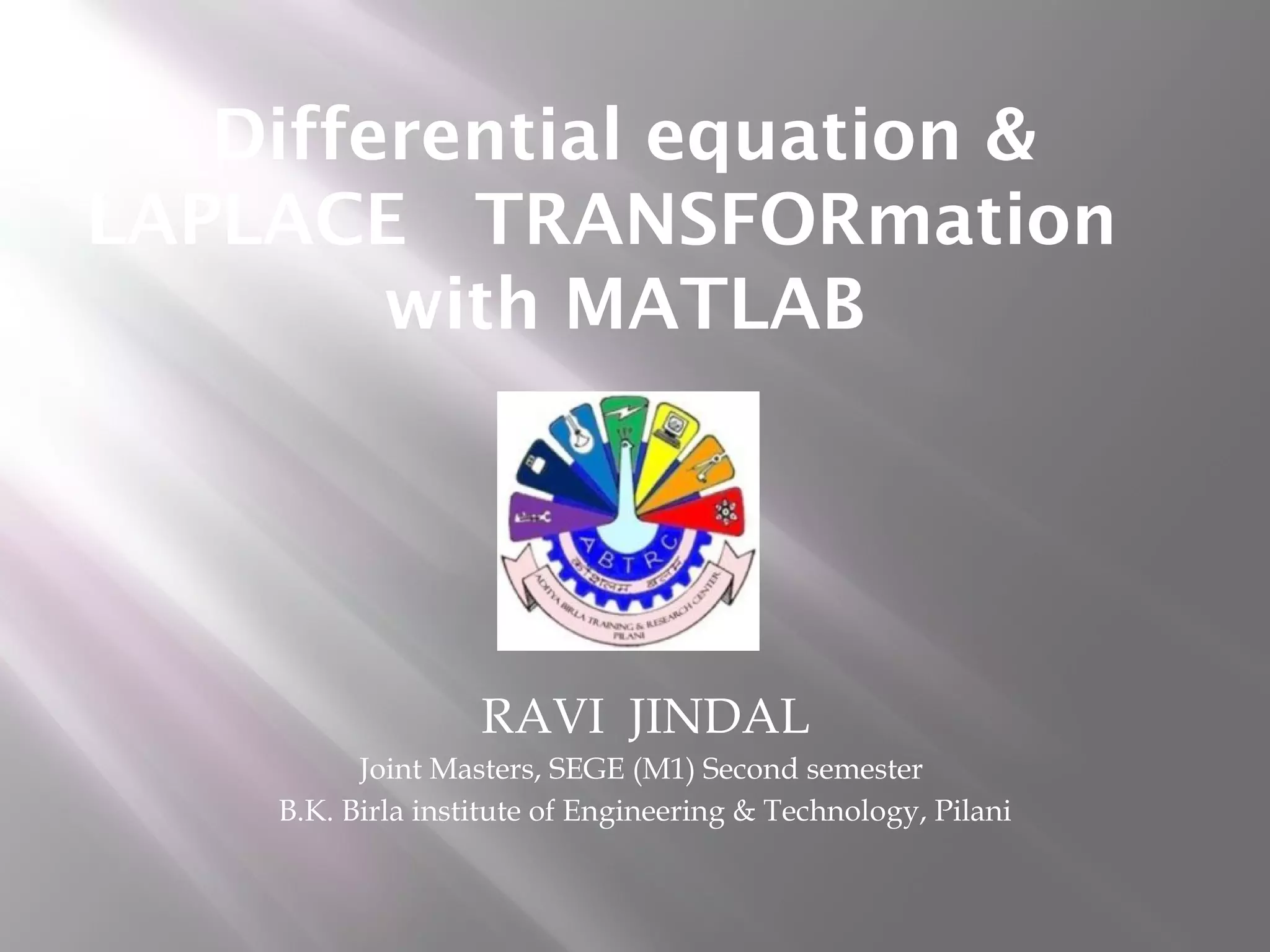
» syms x y t
» [x,y]=dsolve('Dx=3*x+4*y','Dy=-4*x+3*y')
x = exp(3*t)*(cos(4*t)*C1+sin(4*t)*C2)
y = -exp(3*t)*(sin(4*t)*C1-cos(4*t)*C2)
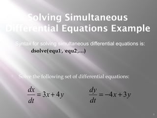
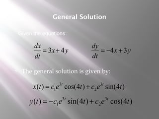
yx
dt
dx
43 += yx
dt
dy
34 +−=
Given the
equations:
General
solution is:
)4sin()4cos()( 3
2
3
1 tectectx tt
+=
)4cos()4sin()( 3
2
3
1 tectecty tt
+−=](https://image.slidesharecdn.com/differentialequationlaplacetransformationwithmatlab-140415045349-phpapp01/85/Differential-equation-laplace-transformation-with-matlab-11-320.jpg)
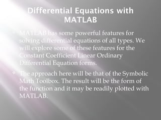
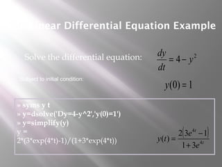
![ Solve the previous system with the initial conditions:
Initial Conditions
0)0( =x 1)0( =y
» [x,y]=dsolve('Dx=3*x+4*y','Dy=-4*x+3*y',
'y(0)=1','x(0)=0')
x = exp(3*t)*sin(4*t)
y = exp(3*t)*cos(4*t) )4cos(
)4sin(
3
3
tey
tex
t
t
=
=](https://image.slidesharecdn.com/differentialequationlaplacetransformationwithmatlab-140415045349-phpapp01/85/Differential-equation-laplace-transformation-with-matlab-12-320.jpg)

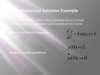
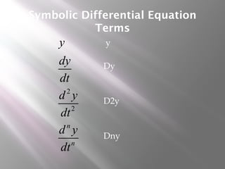
![17
Solve DE with MATLAB.
>> y = dsolve ('D2y + 3*Dy + 2*y = 24',
'y(0)=10', 'Dy(0)=0')
y = 12+2*exp(-2*t)-4*exp(-t)
>> ezplot(y, [0 6])
2
2
3 2 24
d y dy
y
dt dt
+ + =
(0) 10y = '(0) 0y =](https://image.slidesharecdn.com/differentialequationlaplacetransformationwithmatlab-140415045349-phpapp01/85/Differential-equation-laplace-transformation-with-matlab-17-320.jpg)
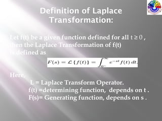
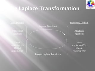
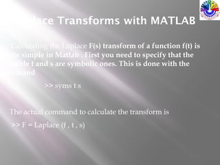
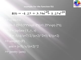
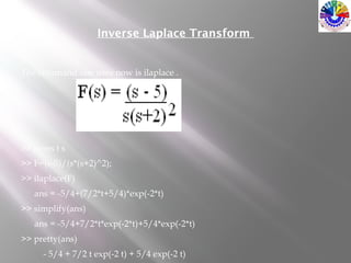


This document discusses using MATLAB to solve differential equations through Laplace transformations. It introduces key terms like the Laplace operator and generating function. It then demonstrates how to use MATLAB commands like "laplace" and "ilaplace" to calculate the Laplace transform of a function and take the inverse Laplace transform. Examples are provided, such as finding the Laplace transform of the function f(t)=-1.25+3.5t*exp(-2t)+1.25*exp(-2t).