Downloaded 52 times
![BMM 104: ENGINEERING MATHEMATICS I Page 1 of 8
CHAPTER 9: THE LAPLACE TRANSFORM
Laplace Transformation and its Inverse
Definition:
Let f (t ) be defined for 0 ≤ t ≤ ∞ and let s denote an arbitrary real variable. The
Laplace transform of f (t ) , designated by either L[ f ( t ) ] or F ( s ) , is
∞
F ( s ) = L[ f (t )] = ∫e −st f (t )dt
0
for all values of s for which the improper integral converges. Convergence occurs when
the limit
∞ a
∫e
−st
f ( t ) dt = lim ∫ e −st f ( t ) dt
a→∞
0 0
exists. If the limit does not exist, the improper integral does not exist, the improper
integral diverges and f (t ) has no Laplace transform. When evaluating the integral, the
variable s is treated as a constant because the integration is with respect to t.
On the other hand, we may write f ( t ) = L−1 [ F ( s ) ] with L−1 is called inverse Laplace
transformation operator and f (t ) is called the inverse Laplace transformation for
F (s) .
Example:
Find the Laplace transform by definition.
(a) L[1] (b) [ ]
L e at
Properties ( Linearity of Laplace Operator L and its inverse L−1 )
Suppose c1 and c 2 are arbitrary constants, then
(i) L{ c1 f 1 ( t ) + c 2 f 2 ( t ) } = c1 L{ f 1 ( t ) } + c 2 L{ f 2 ( t ) } = c1 F1 ( s ) + c 2 F2 ( s )
(ii) L−1 { c1 F1 ( s ) + c 2 F2 ( s )} = c1 L−1 { F1 ( s )} + c 2 L−1 { F2 ( s )} = c1 f 1 ( t ) + c 2 f 2 ( t )
Example:](https://image.slidesharecdn.com/chapter9laplacetransform-130305120725-phpapp01/85/Chapter-9-laplace-transform-1-320.jpg)


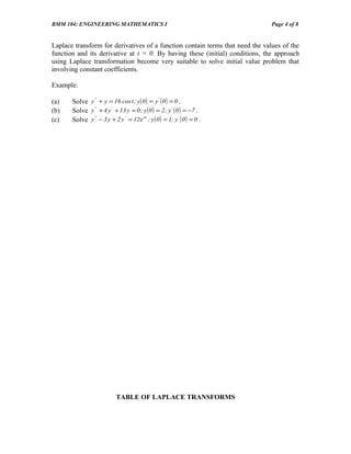


This document provides an overview of the Laplace transform and its properties and applications. Specifically, it defines the Laplace transform and inverse Laplace transform, lists several Laplace transform pairs, and provides examples of using the Laplace transform to solve initial value problems involving differential equations with constant coefficients. It also includes a problem set with exercises calculating Laplace transforms and using them to solve initial value problems.