21 3 ztransform

z-Transforms and
Difference Equations

21.3
Introduction
In this we apply z-transforms to the solution of certain types of difference equation. We shall see that
this is done by turning the difference equation into an ordinary algebraic equation. We investigate
both first and second order difference equations.
A key aspect in this process in the inversion of the z-transform. As well as demonstrating the use of
partial fractions for this purpose we show an alternative, often easier, method using what are known
as residues.
'

$
%
Prerequisites
Before starting this Section you should . . .
• have studied carefully Section 21.2
• be familiar with simple partial fractions
5
4
2
3
Learning Outcomes
On completion you should be able to . . .
• invert z-transforms using partial fractions or
residues where appropriate
• solve constant coefficient linear difference
equations using z-transforms
36 HELM (2005):
Workbook 21: z-Transforms

1. Solution of difference equations using z-transforms
Using z-transforms, in particular the shift theorems discussed at the end of the previous Section,
provides a useful method of solving certain types of difference equation. In particular linear constant
coefficient difference equations are amenable to the z-transform technique although certain other
types can also be tackled. In fact all the difference equations that we looked at in Section 21.1 were
linear:
yn+1 = yn + d (1st order)
yn+1 = A yn (1st order)
yn+2 = yn+1 + yn (2nd order)
Other examples of linear difference equations are
yn+2 + 4yn+1 − 3yn = n2
(2nd order)
yn+1 + yn = n 3n
(1st order)
The key point is that for a difference equation to be classified as linear the terms of the sequence
{yn} arise only to power 1 or, more precisely, the highest subscript term is obtainable as a linear
combination of the lower ones. All the examples cited above are consequently linear. Note carefully
that the term n2
in our fourth example does not imply non-linearity since linearity is determined by
the yn terms.
Examples of non-linear difference equations are
yn+1 = yn + 1
y2
n+1 + 2 yn = 3
yn+1yn = n
cos(yn+1) = yn
We shall not consider the problem of solving non-linear difference equations.
The five linear equations listed above also have constant coefficients; for example:
yn+2 + 4yn+1 − 3yn = n2
has the constant coefficients 1, 4, −3.
The (linear) difference equation
n yn+2 − yn+1 + yn = 0
has one variable coefficient viz n and so is not classified as a constant coefficient difference equation.
Solution of first order linear constant coefficient difference equations
Consider the first order difference equation
yn+1 − 3yn = 4 n = 0, 1, 2, . . .
The equation could be solved in a step-by-step or recursive manner, provided that y0 is known
because
y1 = 4 + 3y0 y2 = 4 + 3y1 y3 = 4 + 3y2 and so on.
This process will certainly produce the terms of the solution sequence {yn} but the general term yn
may not be obvious.
HELM (2005):
Section 21.3: z-Transforms and Difference Equations
37

So consider
yn+1 − 3yn = 4 n = 0, 1, 2, . . . (1)
with initial condition y0 = 1.
We multiply both sides of (1) by z−n
and sum each side over all positive integer values of n and
zero. We obtain
∞
n=0
(yn+1 − 3yn)z−n
=
∞
n=0
4z−n
or
∞
n=0
yn+1z−n
− 3
∞
n=0
ynz−n
= 4
∞
n=0
z−n
(2)
The three terms in (2) are clearly recognisable as z-transforms.
The right-hand side is the z-transform of the constant sequence {4, 4, . . .} which is
4z
z − 1
.
If Y (z) =
∞
n=0
ynz−n
denotes the z-transform of the sequence {yn} that we are seeking then
∞
n=0
yn+1z−n
= z Y (z) − zy0 (by the left shift theorem).
Consequently (2) can be written
z Y (z) − zy0 − 3 Y (z) =
4z
z − 1
(3)
Equation (3) is the z-transform of the original difference equation (1). The intervening steps have
been included here for explanation purposes but we shall omit them in future. The important point
is that (3) is no longer a difference equation. It is an algebraic equation where the unknown, Y (z),
is the z-transform of the solution sequence {yn}.
We now insert the initial condition y0 = 1 and solve (3) for Y (z):
(z − 3)Y (z) − z =
4z
(z − 1)
(z − 3)Y (z) =
4z
z − 1
+ z =
z2
+ 3z
z − 1
so Y (z) =
z2
+ 3z
(z − 1)(z − 3)
(4)
The final step consists of obtaining the sequence {yn} of which (4) is the z-transform. As it stands
(4) is not recognizable as any of the standard transforms that we have obtained. Consequently, one
method of ‘inverting’ (4) is to use a partial fraction expansion. (We assume that you are familiar
with simple partial fractions. See 3.6)
38 HELM (2005):

Thus
Y (z) = z
(z + 3)
(z − 1)(z − 3)
= z
−2
z − 1
+
3
z − 3
(in partial fractions)
so Y (z) =
−2z
z − 1
+
3z
z − 3
Now, taking inverse z-transforms, the general term yn is, using the linearity property,
yn = −2Z−1
{
z
z − 1
} + 3 Z−1
{
z
z − 3
}
The symbolic notation Z−1
is common and is short for ‘the inverse z-transform of’.
TaskTask
Using standard z-transforms write down yn explicitly, where
yn = −2Z−1
{
z
z − 1
} + 3 Z−1
{
z
z − 3
}
Your solution
Answer
yn = −2 + 3 × 3n
= −2 + 3n+1
n = 0, 1, 2, . . . (5)
Checking the solution:
From this solution (5)
yn = −2 + 3n+1
we easily obtain
y0 = −2 + 3 = 1 (as given)
y1 = −2 + 32
= 7
y2 = −2 + 33
= 25
y3 = −2 + 34
= 79 etc.
HELM (2005):
39

These agree with those obtained by recursive solution of the given problem (1):
yn+1 − 3yn = 4 y0 = 1
which yields
y1 = 4 + 3y0 = 7
y2 = 4 + 3y1 = 25
y3 = 4 + 3y2 = 79 etc.
More conclusively we can put the solution (5) back into the left-hand side of the difference equation
(1).
If yn = −2 + 3n+1
then 3yn = −6 + 3n+2
and yn+1 = −2 + 3n+2
So, on the left-hand side of (1),
yn+1 − 3yn = −2 + 3n+2
− (−6 + 3n+2
)
which does indeed equal 4, the given right-hand side, and so the solution has been verified.
Key Point 13
To solve a linear constant coefficient difference equation, three steps are involved:
1. Replace each term in the difference equation by its z-transform and insert the initial condi-
tion(s).
2. Solve the resulting algebraic equation. (Thus gives the z-transform Y (z) of the solution
sequence.)
3. Find the inverse z-transform of Y (z).
The third step is usually the most difficult. We will consider the problem of finding inverse z-
transforms more fully later.
40 HELM (2005):

TaskTask
Solve the diﬀerence equation
yn+1 − yn = d n = 0, 1, 2, . . . y0 = a (6)
where a and d are constants.
(The solution will give the n th
term of an arithmetic sequence with a constant
diﬀerence d and initial term a.)
Start by replacing each term of (6) by its z-transform:
Your solution
Answer
If Y (z) = Z{yn} we obtain the algebraic equation
z Y (z) − zy0 − Y (z) =
d × z
(z − 1)
Note that the right-hand side transform is that of a constant sequence {d, d, . . .}. Note also the
use of the left shift theorem.
Now insert the initial condition y0 = a and then solve for Y (z):
Your solution
HELM (2005):
41

Answer
(z − 1)Y (z) =
d × z
(z − 1)
+ z × a
Y (z) =
d × z
(z − 1)2
+
a × z
z − 1
Finally take the inverse z-transform of the right-hand side. [Hint: Recall the z-transform of the ramp
sequence {n}.]
Your solution
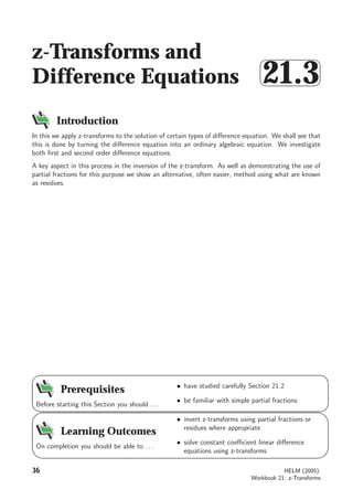
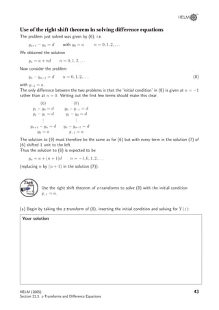
Answer
We have
yn = d × Z−1
{
z
(z − 1)2
} + a × Z−1
{
z
z − 1
}
∴ yn = dn + a n = 0, 1, 2, . . . (7)
using the known z-transforms of the ramp and unit step sequences. Equation (7) may well be a
familiar result to you – an arithmetic sequence whose ‘zeroth’ term is y0 = a has general term
yn = a + nd.
i.e. {yn} = {a, a + d, . . . a + nd, . . .}
This solution is of course readily obtained by direct recursive solution of (6) without need for z-
transforms. In this case the general term (a + nd) is readily seen from the form of the recursive
solution: (Make sure you really do see it).
N.B. If the term a is labelled as the ﬁrst term (rather than the zeroth) then
y1 = a, y2 = a + d, y3 − a + 2d,
so in this case the n th
term is
yn = a + (n − 1)d
rather than (7).
42 HELM (2005):

Use of the right shift theorem in solving difference equations
The problem just solved was given by (6), i.e.
yn+1 − yn = d with y0 = a n = 0, 1, 2, . . .
We obtained the solution
yn = a + nd n = 0, 1, 2, . . .
Now consider the problem
yn − yn−1 = d n = 0, 1, 2, . . . (8)
with y−1 = a.
The only diﬀerence between the two problems is that the ‘initial condition’ in (8) is given at n = −1
rather than at n = 0. Writing out the ﬁrst few terms should make this clear.
(6) (8)
y1 − y0 = d y0 − y−1 = d
y2 − y1 = d y1 − y0 = d
...
...
yn+1 − yn = d yn − yn−1 = d
y0 = a y−1 = a
The solution to (8) must therefore be the same as for (6) but with every term in the solution (7) of
(6) shifted 1 unit to the left.
Thus the solution to (8) is expected to be
yn = a + (n + 1)d n = −1, 0, 1, 2, . . .
(replacing n by (n + 1) in the solution (7)).
TaskTask
Use the right shift theorem of z-transforms to solve (8) with the initial condition
y−1 = a.
(a) Begin by taking the z-transform of (8), inserting the initial condition and solving for Y (z):
Your solution
HELM (2005):
43

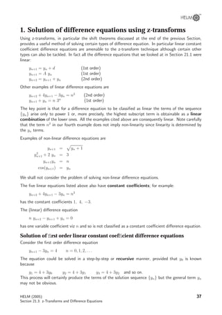
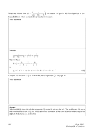
Answer
We have, for the z-transform of (8)
Y (z) − (z−1
Y (z) + y−1) =
dz
z − 1
[Note that here dz means d × z]
Y (z)(1 − z−1
) − a =
dz
z − 1
Y (z)
z − 1
z
=
dz
(z − 1)
+ a
Y (z) =
dz2
(z − 1)2
+
az
z − 1
(9)
The second term of Y (z) has the inverse z-transform {a un} = {a, a, a, . . .}.
The ﬁrst term is less straightforward. However, we have already reasoned that the other term in yn
here should be (n + 1)d.
(b) Show that the z-transform of (n + 1)d is
dz2
(z − 1)2
. Use the standard transform of the ramp and
step:
Your solution
Answer
We have
Z{(n + 1)d} = dZ{n} + dZ{1}
by the linearity property
∴ Z{(n + 1)d} =
dz
(z − 1)2
+
dz
z − 1
= dz
1 + z − 1
(z − 1)2
=
dz2
(z − 1)2
as expected.
44 HELM (2005):

(c) Finally, state yn:
Your solution
Answer
Returning to (9) the inverse z-transform is
yn = (n + 1)d + a un i.e. yn = a + (n + 1)d n = −1, 0, 1, 2, . . .
as we expected.
TaskTask
Earlier in this Section (pages 37-39) we solved
yn+1 − 3yn = 4 n = 0, 1, 2, . . . with y0 = 1.
Now solve yn − 3yn−1 = 4 n = 0, 1, 2, . . . with y−1 = 1. (10)
Begin by obtaining the z-transform of yn:
Your solution
Answer
We have, taking the z-transform of (10),
Y (z) − 3(z−1
Y (z) + 1) =
4z
z − 1
(using the right shift property and inserting the initial condition.)
∴ Y (z) − 3z−1
Y (z) = 3 +
4z
z − 1
Y (z)
(z − 3)
z
= 3 +
4z
z − 1
so Y (z) =
3z
z − 3
+
4z2
(z − 1)(z − 3)
HELM (2005):
45

Write the second term as 4z
z
(z − 1)(z − 3)
and obtain the partial fraction expansion of the
bracketed term. Then complete the z-transform inversion.
Your solution
Answer
z
(z − 1)(z − 3)
=
−1
2
z − 1
+
3
2
z − 3
We now have
Y (z) =
3z
z − 3
−
2z
z − 1
+
6z
z − 3
so
yn = 3 × 3n
− 2 + 6 × 3n
= −2 + 9 × 3n
= −2 + 3n+2
(11)
Compare this solution (11) to that of the previous problem (5) on page 39:
Your solution
Answer
Solution (11) is just the solution sequence (5) moved 1 unit to the left. We anticipated this since
the diﬀerence equation (10) and associated initial condition is the same as the diﬀerence equation
(1) but shifted one unit to the left.
46 HELM (2005):

2. Second order difference equations
You will learn in this section about solving second order linear constant coefficient difference equations.
In this case two initial conditions are required, typically either y0 and y1 or y−1 and y−2. In the first
case we use the left shift property of the z-transform, in the second case we use the right shift
property. The same three basic steps are involved as in the first order case.
TaskTask
By solving
yn+2 = yn+1 + yn (12)
y0 = y1 = 1
obtain the general term yn of the Fibonacci sequence.
Begin by taking the z-transform of (12), using the left shift property. Then insert the initial conditions
and solve the resulting algebraic equation for Y (z), the z-transform of {yn}:
Your solution
Answer
z2
Y (z) − z2
y0 − zy1 = zY (z) − zy0 + Y (z) (taking z-transforms )
z2
Y (z) − z2
− z = zY (z) − z + Y (z) (inserting initial conditions)
(z2
− z − 1)Y (z) = z2
so
Y (z) =
z2
z2 − z − 1
(solving for Y (z)).
HELM (2005):
47

Now solve the quadratic equation z2
− z − 1 = 0 and hence factorize the denominator of Y (z):
Your solution
Answer
z2
− z − 1 = 0
∴ z =
1 ±
√
1 + 4
2
=
1 ±
√
5
2
so if a =
1 +
√
5
2
, b =
1 −
√
5
2
Y (z) =
z2
(z − a)(z − b)
This form for Y (z) often arises in solving second order diﬀerence equations. Write it in partial
fractions and ﬁnd yn, leaving a and b as general at this stage:
Your solution
Answer
Y (z) = z
z
(z − a)(z − b)
=
Az
z − a
+
Bz
(z − b)
in partial fractions
where A =
a
a − b
and B =
b
b − a
Hence, taking inverse z-transforms
yn = Aan
+ Bbn
=
1
(a − b)
(an+1
− bn+1
) (13)
48 HELM (2005):

Now complete the Fibonacci problem:
Your solution
Answer
With a =
1 +
√
5
2
b =
1 −
√
5
2
so a − b =
√
5
we obtain, using (13)
yn =
1
√
5

 1 +
√
5
2
n+1
−
1 −
√
5
2
n

 n = 2, 3, 4, . . .
for the n th
term of the Fibonacci sequence.
With an appropriate computational aid you could (i) check that this formula does indeed give the
familiar sequence
{1, 1, 2, 3, 5, 8, 13, . . .}
and (ii) obtain, for example, y50 and y100.
Key Point 14
The inverse z-transform of
Y (z) =
z2
(z − a)(z − b)
a = b is yn =
1
(a − b)
(an+1
− bn+1
)
HELM (2005):
49

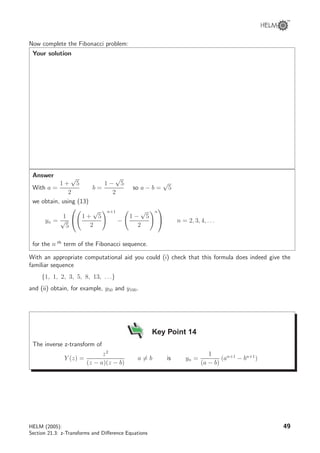
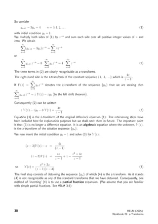
TaskTask
Use the right shift property of z-transforms to solve the second order diﬀerence
equation
yn − 7yn−1 + 10 yn−2 = 0 with y−1 = 16 and y−2 = 5.
[Hint: the steps involved are the same as in the previous Task]
Your solution
Answer
Y (z) − 7(z−1
Y (z) + 16) + 10(z−2
Y (z) + 16z−1
+ 5) = 0
Y (z)(1 − 7z−1
+ 10z−2
) − 112 + 160z−1
+ 50 = 0
Y (z)
z2
− 7z + 10
z2
= 62 − 160z−1
Y (z) =
62z2
z2 − 7z + 10
−
160z
z2 − 7z + 10
= z
(62z − 160)
(z − 2)(z − 5)
=
12z
z − 2
+
50z
z − 5
so yn = 12 × 2n
+ 50 × 5n
n = 0, 1, 2, . . .
We now give an Example where a quadratic equation with repeated solutions arises.
50 HELM (2005):

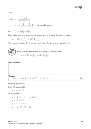
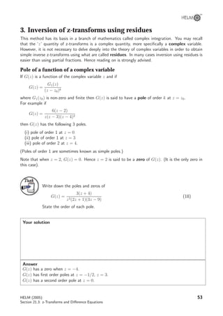
Example 1
(a) Obtain the z-transform of {fn} = {nan
}.
(b) Solve
yn − 6yn−1 + 9yn−2 = 0 n = 0, 1, 2, . . .
y−1 = 1 y−2 = 0
[Hint: use the result from (a) at the inversion stage.]
Solution
(a) Z{n} =
z
(z − 1)2
∴ Z{nan
} =
z/a
(z/a − 1)2 =
az
(z − a)2
where we have used the
property Z{fn an
} = F
z
a
(b) Taking the z-transform of the diﬀerence equation and inserting the initial conditions:
Y (z) − 6(z−1
Y (z) + 1) + 9(z−2
Y (z) + z−1
) = 0
Y (z)(1 − 6z−1
+ 9z−2
) = 6 − 9z−1
Y (z)(z2
− 6z + 9) = 6z2
− 9z
Y (z) =
6z2
− 9z
(z − 3)2
= z
6z − 9
(z − 3)2
= z
6
z − 3
+
9
(z − 3)2
from which, using the result (a) on the second term,
yn = 6 × 3n
+ 3n × 3n
= (6 + 3n)3n
We shall re-do this inversion by an alternative method shortly.
TaskTask
Solve the diﬀerence equation
yn+2 + yn = 0 with y0, y1 arbitrary. (14)
Start by obtaining Y (z) using the left shift theorem:
Your solution
HELM (2005):
51

Answer
z2
Y (z) − z2
y0 − zy1 + Y (z) = 0
(z2
+ 1)Y (z) = z2
y0 + zy1
Y (z) =
z2
z2 + 1
y0 +
z
z2 + 1
y1
To find the inverse z-transforms recall the results for Z{cos ωn} and Z{sin ωn} from Key Point 6
(page 21) and some of the particular cases discussed in Section 21.2. Hence find yn here:
Your solution
Answer
Taking Z{cos ωn} and Z{sin ωn} with ω =
π
2
Z cos
nπ
2
=
z2
z2 + 1
Z sin
nπ
2
=
z
z2 + 1
Hence yn = y0Z−1
{
z2
z2 + 1
} + y1Z−1
{
z
z2 + 1
} = y0 cos
nπ
2
+ y1 sin
nπ
2
(15)
Those of you who are familiar with differential equations may know that
d2
y
dt2
+ y = 0 y(0) = y0, y (0) = y0 (16)
has solutions y1 = cos t and y2 = sin t and a general solution
y = c1 cos t + c2 sin t (17)
where c1 = y0 and c2 = y0.
This differential equation is a model for simple harmonic oscillations. The difference equation (14)
and its solution (15) are the discrete counterparts of (16) and (17).
52 HELM (2005):

3. Inversion of z-transforms using residues
This method has its basis in a branch of mathematics called complex integration. You may recall
that the ‘z’ quantity of z-transforms is a complex quantity, more specifically a complex variable.
However, it is not necessary to delve deeply into the theory of complex variables in order to obtain
simple inverse z-transforms using what are called residues. In many cases inversion using residues is
easier than using partial fractions. Hence reading on is strongly advised.
Pole of a function of a complex variable
If G(z) is a function of the complex variable z and if
G(z) =
G1(z)
(z − z0)k
where G1(z0) is non-zero and finite then G(z) is said to have a pole of order k at z = z0.
For example if
G(z) =
6(z − 2)
z(z − 3)(z − 4)2
then G(z) has the following 3 poles.
(i) pole of order 1 at z = 0
(ii) pole of order 1 at z = 3
(iii) pole of order 2 at z = 4.
(Poles of order 1 are sometimes known as simple poles.)
Note that when z = 2, G(z) = 0. Hence z = 2 is said to be a zero of G(z). (It is the only zero in
this case).
TaskTask
Write down the poles and zeros of
G(z) =
3(z + 4)
z2(2z + 1)(3z − 9)
(18)
State the order of each pole.
Your solution
Answer
G(z) has a zero when z = −4.
G(z) has first order poles at z = −1/2, z = 3.
G(z) has a second order pole at z = 0.
HELM (2005):
53

Residue at a pole
The residue of a complex function G(z) at a first order pole z0 is
Res (G(z), z0) = [G(z)(z − z0)]z0
(19)
The residue at a second order pole z0 is
Res (G(z), z0) =
d
dz
(G(z)(z − z0)2
)
z0
(20)
You need not worry about how these results are obtained or their full mathematical significance.
(Any textbook on Complex Variable Theory could be consulted by interested readers.)
Example
Consider again the function (18) in the previous guided exercise.
G(z) =
3(z + 4)
z2(2z + 1)(3z − 9)
=
(z + 4)
2z2 z + 1
2
(z − 3)
The second form is the more convenient for the residue formulae to be used.
Using (19) at the two first order poles:
Res G(z), −
1
2
= G(z) z − −
1
2 1
2
=
(z + 4)
2z2(z − 3) 1
2
= −
18
5
Res [G(z), 3] =




(z + 4)
2z2 z +
1
2




3
=
1
9
Using (20) at the second order pole
Res (G(z), 0) =
d
dz
(G(z)(z − 0)2
)
0
The differentiation has to be carried out before the substitution of z = 0 of course.
∴ Res (G(z), 0) =




d
dz




(z + 4)
2 z +
1
2
(z − 3)








0
=
1
2



d
dz



z + 4
z2 −
5
2
z −
3
2






0
54 HELM (2005):

TaskTask
Carry out the differentiation shown on the last line of the previous page, then
substitute z = 0 and hence obtain the required residue.
Your solution
Answer
Differentiating by the quotient rule then substituting z = 0 gives
Res (G(z), 0) =
17
9
Key Point 15
Residue at a Pole of Order kkk
If G(z) has a kth
order pole at z = z0
i.e. G(z) =
G1(z)
(z − z0)k
G1(z0) = 0 and finite
Res (G(z), z0) =
1
(k − 1)!
dk−1
dzk−1
(G(z) (z − z0)k
)
z0
(21)
This formula reduces to (19) and (20) when k = 1 and 2 respectively.
HELM (2005):
55

Inverse z-transform formula
Recall that, by deﬁnition, the z-transform of a sequence {fn} is
F(z) = f0 + f1z−1
+ f2z−2
+ . . . fnz−n
+ . . .
If we multiply both sides by zn−1
where n is a positive integer we obtain
F(z)zn−1
= f0zn−1
+ f1zn−2
+ f2zn−3
+ . . . fnz−1
+ fn+1z−2
+ . . .
Using again a result from complex integration it can be shown from this expression that the general
term fn is given by
fn = sum of residues of F(z) zn−1
at its poles (22)
The poles of F(z)zn−1
will be those of F(z) with possibly additional poles at the origin.
To illustrate the residue method of inversion we shall re-do some of the earlier examples that were
done using partial fractions.
Example:
Y (z) =
z2
(z − a)(z − b)
a = b
so
Y (z)zn−1
=
zn+1
(z − a)(z − b)
= G(z), say.
G(z) has ﬁrst order poles at z = a, z = b so using (19).
Res (G(z), a) =
zn+1
z − b a
=
an+1
a − b
Res (G(z), b) =
zn+1
z − a b
=
bn+1
b − a
=
−bn+1
a − b
We need simply add these residues to obtain the required inverse z-transform
∴ fn =
1
(a − b)
(an+1
− bn+1
)
as before.
56 HELM (2005):

TaskTask
Obtain, using (22), the inverse z-transform of
Y (z) =
6z2
− 9z
(z − 3)2
Firstly, obtain the pole(s) of G(z) = Y (z)zn−1
and deduce the order:
Your solution
Answer
G(z) = Y (z)zn−1
=
6zn+1
− 9zn
(z − 3)2
whose only pole is one of second order at z = 3.
Now calculate the residue of G(z) at z = 3 using (20) and hence write down the required inverse
z-transform yn:
Your solution
HELM (2005):
57

Answer
Res (G(z), 3) =
d
dz
(6zn+1
− 9zn
)
3
= 6(n + 1)zn
− 9nzn−1
3
= 6(n + 1)3n
− 9n3n−1
= 6 × 3n
+ 3n3n
This is the same as was found by partial fractions, but there is considerably less labour by the residue
method.
In the above examples all the poles of the various functions G(z) were real. This is the easiest
situation but the residue method will cope with complex poles.
Example
We showed earlier that
z2
z2 + 1
and cos
nπ
2
formed a z-transform pair.
We will now obtain yn if Y (z) =
z2
z2 + 1
using residues.
Using residues with, from (22),
G(z) =
zn+1
z2 + 1
=
zn+1
(z − i)(z + i)
where i2
= −1.
we see that G(z) has ﬁrst order poles at the complex conjugate points ± i.
Using (19)
Res (G(z), i) =
zn+1
z + i i
=
in+1
2i
Res (G(z), −i) =
(−i)n+1
(−2i)
(Note the complex conjugate residues at the complex conjugate poles.)
Hence Z−1
{
z2
z2 + 1
} =
1
2i
in+1
− (−i)n+1
But i = eiπ/2
and −i = e−iπ/2
, so the inverse z-transform is
1
2i
ei(n+1)π/2
− e−i(n+1)π/2
= sin(n + 1)
π
2
= cos
nπ
2
as expected.
58 HELM (2005):

TaskTask
Show, using residues, that
Z−1
{
z
z2 + 1
} = sin
nπ
2
Your solution
Answer
Using (22):
G(z) = zn−1 z
z2 + 1
=
zn
z2 + 1
=
zn
(z + i)(z − i)
Res (G(z), i) =
in
2i
Res (G(z), −i) =
(−i)n
−2i
Z−1
{
z
z2 + 1
} =
1
2i
(in
− (−i)n
)
=
1
2i
(einπ/2
− e−inπ/2
)
= sin
nπ
2
HELM (2005):
59

4. An application of difference equations – currents in a
ladder network
The application we will consider is that of finding the electric currents in each loop of the ladder resis-
tance network shown, which consists of (N + 1) loops. The currents form a sequence {i0, i1, . . . iN }
V io i1 in in+1 iN
Figure 7
All the resistors have the same resistance R so loops 1 to N are identical. The zero’th loop contains
an applied voltage V . In this zero’th loop, Kirchhoff’s voltage law gives
V = Ri0 + R(i0 − i1)
from which
i1 = 2i0 −
V
R
(23)
Similarly, applying the Kirchhoff law to the (n + 1)th
loop where there is no voltage source and 3
resistors
0 = Rin+1 + R(in+1 − in+2) + R(in+1 − in)
from which
in+2 − 3in+1 + in = 0 n = 0, 1, 2, . . . (N − 2) (24)
(24) is the basic difference equation that has to be solved.
TaskTask
Using the left shift theorems obtain the z-transform of equation (24). Denote by
I(z) the z-transform of {in}. Simplify the algebraic equation you obtain.
Your solution
60 HELM (2005):

Answer
We obtain
z2
I(z) − z2
i0 − zi1 − 3(zI(z) − zi0) + I(z) = 0
Simplifying
(z2
− 3z + 1)I(z) = z2
i0 + zi1 − 3zi0 (25)
If we now eliminate i1 using (23), the right-hand side of (25) becomes
z2
i0 + z 2i0 −
V
R
− 3zi0 = z2
i0 − zi0 − z
V
R
= i0 z2
− z − z
V
i0R
Hence from (25)
I(z) =
i0 z2
− 1 +
V
i0R
z
z2 − 3z + 1
(26)
Our ﬁnal task is to ﬁnd the inverse z-transform of (26).
TaskTask
Look at the table of z-transforms on page 35 (or at the back of the Workbook)
and suggest what sequences are likely to arise by inverting I(z) as given in (26).
Your solution
Answer
The most likely candidates are hyperbolic sequences because both {cosh αn} and {sinh αn} have
z-transforms with denominator
z2
− 2z cosh α + 1
which is of the same form as the denominator of (26), remembering that cosh α ≥ 1. (Why are the
trigonometric sequences {cos ωn} and {sin ωn} not plausible here?)
To proceed, we introduce a quantity α such that α is the positive solution of 2 cosh α = 3 from
which (using cosh2
α − sinh2
α ≡ 1) we get
HELM (2005):
61

sinh α =
9
4
− 1 =
√
5
2
Hence (26) can be written
I(z) = i0
z2
− 1 +
V
i0R
z
z2 − 2z cosh α + 1
(27)
To further progress, bearing in mind the z-transforms of {cosh αn} and {sinh αn}, we must subtract
and add z cosh α to the numerator of (27), where cosh α = 3
2
.
I(z) = i0




z2
− z cosh α +
3z
2
− 1 +
V
i0R
z
z2 − 2z cosh α + 1




= i0




(z2
− z cosh α)
z2 − 2z cosh α + 1
+
3
2
− 1 z −
V z
i0R
z2 − 2z cosh α + 1




The ﬁrst term in the square bracket is the z-transform of {cosh αn}.
The second term is
1
2
−
V
i0R
z
z2 − 2z cosh α + 1
=
1
2
−
V
i0R
2
√
5
z
√
5
2
z2 − 2z cosh α + 1
which has inverse z-transform
1
2
−
V
i0R
2
√
5
sinh αn Hence we have for the loop currents
in = i0 cosh(αn) +
i0
2
−
V
R
2
√
5
sinh(αn) n = 0, 1, . . . N (27)
where cosh α =
3
2
determines the value of α.
Finally, by Kirchhoﬀ’s law applied to the rightmost loop
3iN = iN−1
from which, with (27), we could determine the value of i0.
62 HELM (2005):

Exercises
1. Deduce the inverse z-transform of each of the following functions:
(a)
2z2
− 3z
z2 − 3z − 4
(b)
2z2
+ z
(z − 1)2
(c)
2z2
− z
2z2 − 2z + 2
(d)
3z2
+ 5
z4
2. Use z-transforms to solve each of the following diﬀerence equations:
(a) yn+1 − 3yn = 4n
y0 = 0
(b) yn − 3yn−1 = 6 y−1 = 4
(c) yn − 2yn−1 = n y−1 = 0
(d) yn+1 − 5yn = 5n+1
y0 = 0
(e) yn+1 + 3yn = 4δn−2 y0 = 2
(f) yn − 7yn−1 + 10yn−2 = 0 y−1 = 16, y−2 = 5
(g) yn − 6yn−1 + 9yn−2 = 0 y−1 = 1, y−2 = 0
Answers
1 (a) (−1)n
+ 4n
(b) 2 + 3n (c) cos(nπ/3) (d) 3δn−2 + 5δn−4
2 (a) yn = 4n
− 3n
(b) yn = 21 × 3n
− 3 (c) yn = 2 × 2n
− 2 − n (d) yn = n5n
(e) yn = 2 × (−3)n
+ 4 × (−3)n−3
un−2 (f) yn = 12 × 2n
+ 50 × 5n
(g) yn = (6 + 3n)3n
HELM (2005):
63

21 3 ztransform

Recommended

Recommended

More Related Content

What's hot

What's hot (20)

Similar to 21 3 ztransform

Similar to 21 3 ztransform (20)

Recently uploaded

Recently uploaded (20)

21 3 ztransform