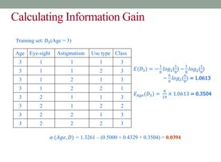
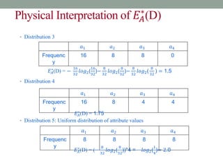
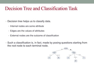
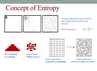
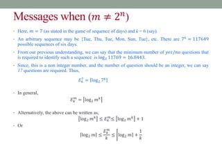
This document discusses decision trees and entropy. It begins by providing examples of binary and numeric decision trees used for classification. It then describes characteristics of decision trees such as nodes, edges, and paths. Decision trees are used for classification by organizing attributes, values, and outcomes. The document explains how to build decision trees using a top-down approach and discusses splitting nodes based on attribute type. It introduces the concept of entropy from information theory and how it can measure the uncertainty in data for classification. Entropy is the minimum number of questions needed to identify an unknown value.
![Illustration : BuildDTAlgorithm
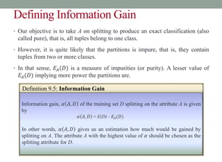
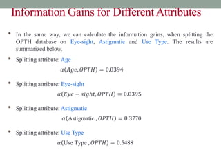
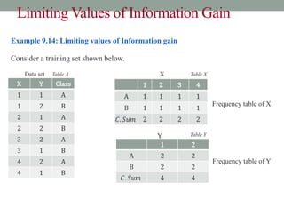
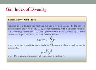
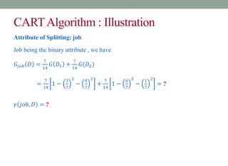
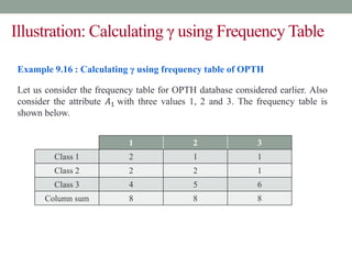
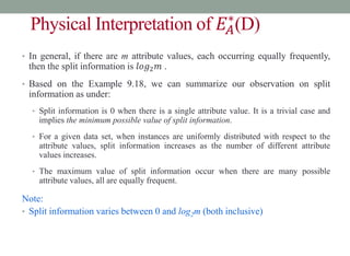
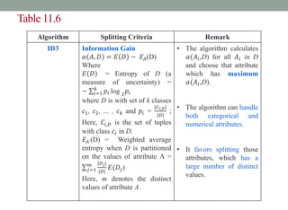
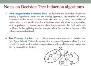
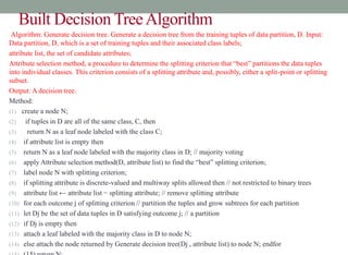
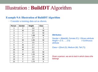
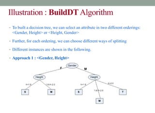
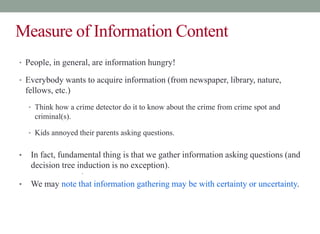
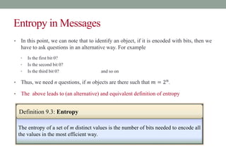
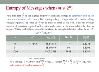
Example 9.5: Illustration of BuildDT Algorithm
• Consider an anonymous database as shown.
A1 A2 A3 A4 Class
a11 a21 a31 a41 C1
a12 a21 a31 a42 C1
a11 a21 a31 a41 C1
a11 a22 a32 a41 C2
a11 a22 a32 a41 C2
a12 a22 a31 a41 C1
a11 a22 a32 a41 C2
a11 a22 a31 a42 C1
a11 a21 a32 a42 C2
a11 a22 a32 a41 C2
a12 a22 a31 a41 C1
a12 a22 a31 a42 C1
• Is there any “clue” that enables to
select the “best” attribute first?
• Suppose, following are two
attempts:
• A1A2A3A4 [naïve]
• A3A2A4A1 [Random]
• Draw the decision trees in the above-
mentioned two cases.
• Are the trees different to classify any test
data?
• If any other sample data is added into the
database, is that likely to alter the decision
tree already obtained?](https://image.slidesharecdn.com/decisiontreeinduction-211002173058/85/Decision-tree-induction-19-320.jpg)
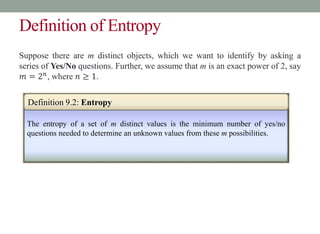
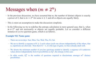
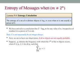

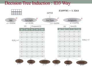
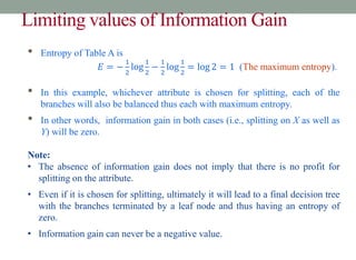
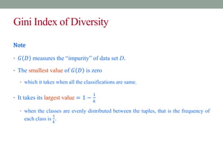
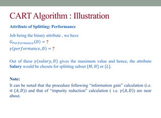
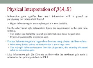
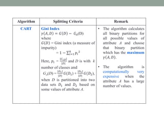
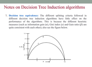
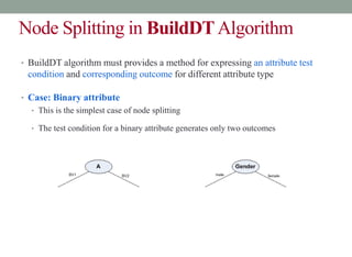
![ID3: Decision Tree InductionAlgorithms
• Quinlan [1986] introduced the ID3, a popular short form of Iterative
Dichotomizer 3 for decision trees from a set of training data.
• In ID3, each node corresponds to a splitting attribute and each arc is a possible
value of that attribute.
• At each node, the splitting attribute is selected to be the most informative
among the attributes not yet considered in the path starting from the root.](https://image.slidesharecdn.com/decisiontreeinduction-211002173058/85/Decision-tree-induction-51-320.jpg)