Download to read offline

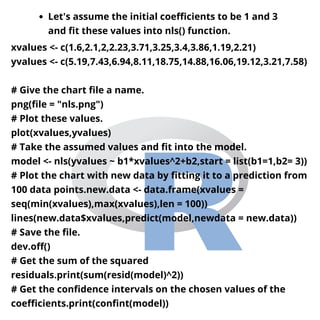
![When we execute the above code, it produces the
following result:-
[1] 1.081935
Waiting for profiling to be done...
2.5% 97.5%
b1 1.137708 1.253135
b2 1.497364 2.496484](https://image.slidesharecdn.com/r-nonlinearleastsquare-211110064132/85/R-nonlinear-least-square-7-320.jpg)


The document discusses nonlinear least squares regression in R. It explains that real-world data is rarely linear and instead follows curves and higher-order mathematical functions. Nonlinear regression aims to find the curve that best fits the data by adjusting the model's parameters. In R, the nls() function is used to estimate the parameters and their confidence intervals for a defined nonlinear model, with the basic syntax being nls(formula, data, start). An example is provided using a quadratic model and nls() to output the sum of squared residuals and confidence intervals for the coefficients.