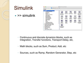
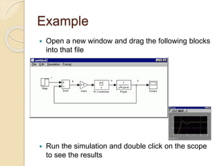
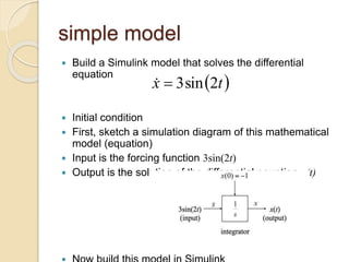
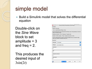
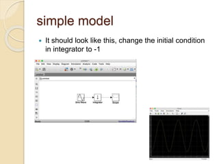
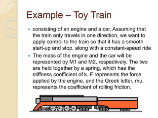
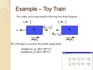
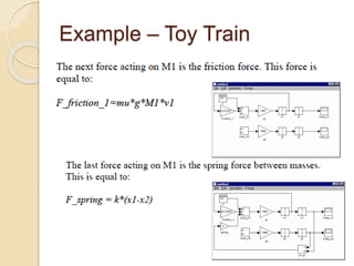
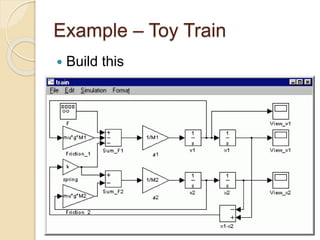
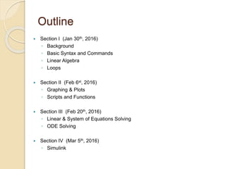
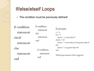
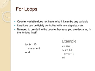
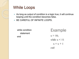
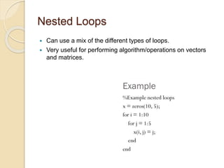
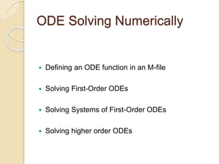
This document provides an outline and overview of topics that will be covered in an introduction to MATLAB and Simulink course over 4 sections. Section I will cover background, basic syntax and commands, linear algebra, and loops. Section II will cover graphing/plots, scripts and functions. Section III will cover solving linear and systems of equations and solving ODEs. Section IV will cover Simulink. The document provides examples of content that will be covered within each section, such as plotting functions, solving systems of equations using matrices, and numerically and symbolically solving ODEs.

![MATLAB Matrices
A matrix with only one row is called a row vector. A row vector can be
created in MATLAB as follows (note the commas):
» rowvec = [12 , 14 , 63]
rowvec =
12 14 63
A matrix with only one column is called a column vector. A column
vector can be created in MATLAB as follows (note the semicolons):
» colvec = [13 ; 45; -2]
colvec =
13
45
-2](https://image.slidesharecdn.com/presentation-230529111938-5bf97206/85/presentation-pptx-9-320.jpg)
![MATLAB Matrices
A matrix can be created in MATLAB as follows (note the commas
AND semicolons):
» matrix = [1 , 2 , 3 ; 4 , 5 ,6 ; 7 , 8 , 9]
matrix =
1 2 3
4 5 6
7 8 9](https://image.slidesharecdn.com/presentation-230529111938-5bf97206/85/presentation-pptx-10-320.jpg)
![Index
MATLAB index starts with 1, NOT 0!
Vector Index:
◦ a = [22 17 7 4 42]
a(1) = 22
a(3) = 7
Matrix Index:
◦ a = [7 12 42; 5 1 23; 4 9 10];
a(1, 3) = 42
a(3, 2) = 9](https://image.slidesharecdn.com/presentation-230529111938-5bf97206/85/presentation-pptx-11-320.jpg)
![Some matrix functions in MATLAB
X = ones(r,c) Creates matrix full with ones
X = zeros(r,c) Creates matrix full with zeros
A = diag(x) Creates squared matrix with vector x in diagonal
[r,c] = size(A) Return dimensions of matrix A
X = A’ Transposed matrix
X = inv(A) Inverse matrix squared matrix
X = pinv(A) Pseudo inverse
d = det(A) Determinant
[X,D] = eig(A) Eigenvalues and eigenvectors
[U,D,V] = svd(A) singular value decomposition](https://image.slidesharecdn.com/presentation-230529111938-5bf97206/85/presentation-pptx-12-320.jpg)
![Dot Operator
For scalar operations, nothing new is needed. Example:
a = 5; b = 3; ==> c = a*b %c = 15
For element operations, a dot must be used before the operator.
Note: Dot operator not the same as dot product!
Example:
◦ a = [1 2 3 4];
◦ b = [5 6 7 8];
◦ c = a*b
◦ Result: ??? Error using ==> mtimes
inner matrix dimensions must agree
Now, try:
◦ c = a.*b %notice the dot!
◦ Result: c=[5 12 21 32]
Notice what it is doing: a(1)*b(1), a(2)*b(2), etc.](https://image.slidesharecdn.com/presentation-230529111938-5bf97206/85/presentation-pptx-13-320.jpg)
![Axis-specific
Helps focus on what is important on the graph.
Change only the x or y axis limits:
◦ xlim([xminxmax]) or ylim([yminymax])
◦ min and max can be positive or negative.
example](https://image.slidesharecdn.com/presentation-230529111938-5bf97206/85/presentation-pptx-26-320.jpg)
![plotyy
2D line plots with y-axis on both left and right side
◦ [AX,H1,H2]=plotyy(x1,y1,x2,y2)](https://image.slidesharecdn.com/presentation-230529111938-5bf97206/85/presentation-pptx-28-320.jpg)
![Polynomials
We can use an array to represent a polynomial. To do so we
use list the coefficients in decreasing order of the powers. For
example x3+4x+15 will look like [1 0 4 15]
To find roots of this polynomial we use roots command. roots
([1 0 4 15])
To create a polynomial from its roots poly command is used.
poly([1 2 3]) where r1=1, r2=2, r3=3
To evaluate the new polynomial at x =5 we can use polyval
command. polyval([ 1 -6 11 -6], 5)](https://image.slidesharecdn.com/presentation-230529111938-5bf97206/85/presentation-pptx-31-320.jpg)
![Systems of Equations
Consider the following system of equations
◦ x+5y+15z=7
◦ x-3y+13z=3
◦ 3x-4y-15z=11
One way to solve this system of equations is to use matrices.
First, define matrix A:
◦ A=[1 5 15; 1 -3 13; 3 -4 15];
Second, matrix b:
◦ b=[7;3;11];
Third, we solve the equation Ax=b for x, taking the inverse of A
and multiply it by b:
◦ x=inv(A)*b
Note that we cannot solve equation Ax=b by dividing b by A
because vectors A and b have different dimensions!](https://image.slidesharecdn.com/presentation-230529111938-5bf97206/85/presentation-pptx-32-320.jpg)
![Systems of Equations
Consider the following system of equations
◦ x+5y+15z=7
◦ x-3y+13z=3
◦ 3x-4y-15z=11
One way to solve this system of equations is to use matrices.
First, define matrix A:
◦ A=[1 5 15; 1 -3 13; 3 -4 15];
Second, matrix b:
◦ b=[7;3;11];
Third, we solve the equation Ax=b for x, taking the inverse of A
and multiply it by b:
◦ x=inv(A)*b
Note that we cannot solve equation Ax=b by dividing b by A
because vectors A and b have different dimensions!](https://image.slidesharecdn.com/presentation-230529111938-5bf97206/85/presentation-pptx-34-320.jpg)
![Solving ODE with dsolve,
systems
Systems of equations
◦ EQs:
[x,y,z]=dsolve(’Dx=x+2*y-z’,’Dy=x+z’,’Dz=4*x-4*y+5*z’)
inits=’x(0)=1,y(0)=2,z(0)=3’;
[x,y,z]=dsolve(’Dx=x+2*y-z’,’Dy=x+z’,’Dz=4*x-4*y+5*z’,inits)
Notice that since no independent variable was specified,
MATLAB used its default, t.
◦ Plotting
t=linspace(0,.5,25);
xx=eval(vectorize(x));
yy=eval(vectorize(y));
zz=eval(vectorize(z));
plot(t, xx, t, yy, t, zz)](https://image.slidesharecdn.com/presentation-230529111938-5bf97206/85/presentation-pptx-39-320.jpg)
![Solving first-order ODEs
Define the function M-file
function y_dot=EOM(y,t)
global alpha gamma
y_dot=alpha * y - gamma * y^2;
end
Make a script M-file
global alpha gamma
alpha=0.15;
gamma=3.5;
y0=1;
[y t]=ode45(@EOM,[0 10],y0);
plot(t,y);](https://image.slidesharecdn.com/presentation-230529111938-5bf97206/85/presentation-pptx-44-320.jpg)
![Example
Use “ode45” to solve the following differential
equation and plot y(x) in the interval of [0,6π]. Put
your name in the plot title.](https://image.slidesharecdn.com/presentation-230529111938-5bf97206/85/presentation-pptx-47-320.jpg)
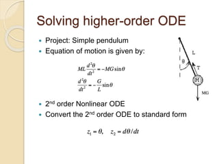
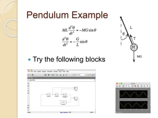
![Simple Pendulum
Initial conditions and constants
Coding
◦ Make a function M-file for equation of motion
function z_dot=EOM_pendulum(t,z)
global G L
theta=z(1);
theta_dot=z(2);
theta_dot2=-(G/L)*sin(theta);
z_dot=[theta_dot;theta_dot2];
end
◦ Make a script M-file to run the code
global G L
G=9.8;
L=2;
tspan=[0 2*pi];
inits=[pi/3 0];
[t, y]=ode45(@EOM_pendulum,tspan,inits);](https://image.slidesharecdn.com/presentation-230529111938-5bf97206/85/presentation-pptx-49-320.jpg)
![Lorenz Equations
Initials and constants, T=[0 20]
Plot x vs. z , check if you
get same results as](https://image.slidesharecdn.com/presentation-230529111938-5bf97206/85/presentation-pptx-50-320.jpg)