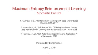
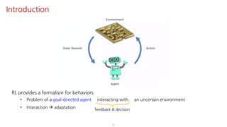
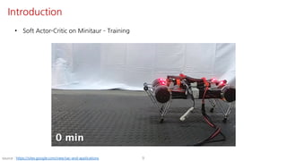
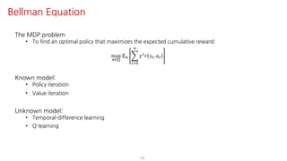
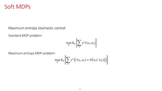
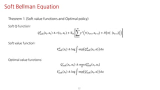
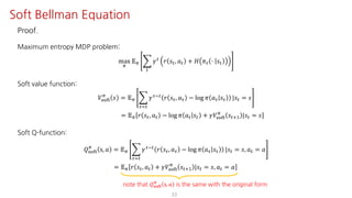
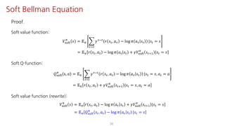
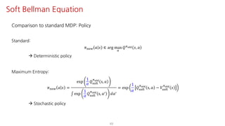
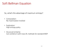
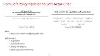
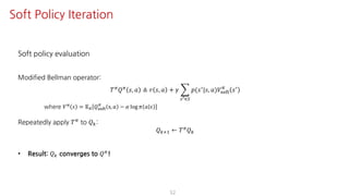
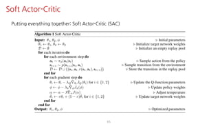
The document presents an overview of maximum entropy reinforcement learning, exploring key concepts such as Markov decision processes, the Bellman equation, and various exploration methods. It highlights the importance of adapting to uncertainty in environments while employing deep learning techniques for policy optimization. The Soft Actor-Critic algorithm is discussed in detail, emphasizing its applications and benefits in reinforcement learning scenarios.

1. 1
Maximum Entropy Reinforcement Learning
Stochastic Control
T. Haarnoja, et al., “Reinforcement Learning with Deep Energy-Based Policies”, ICML
2017
T. Haarnoja, et, al., “Soft Actor-Critic: Off-Policy Maximum Entropy Deep Reinforcement
Learning with a Stochastic Actor”, ICML 2018
T. Haarnoja, et, al., “Soft Actor-Critic Algorithms and Applications”, arXiv preprint 2018
Dongmin Lee
August, 2019
T. Haarnoja, et al., “Reinforcement Learning with Deep Energy-Based
Policies”, ICML 2017
T. Haarnoja, et, al., “Soft Actor-Critic: Off-Policy Maximum Entropy
Deep Reinforcement Learning with a Stochastic Actor”, ICML 2018
T. Haarnoja, et, al., “Soft Actor-Critic Algorithms and Applications”,
arXiv preprint 2018
Presented by Dongmin Lee
August, 2019

2. 2
Outline
1. Introduction
2. Reinforcement Learning
• Markov Decision Processes (MDPs)
• Bellman Equation
3. Exploration methods
4. Maximum Entropy Reinforcement Learning
• Soft MDPs
• Soft Bellman Equation
5. From Soft Policy Iteration to Soft Actor-Critic
• Soft Policy Iteration
• Soft Actor-Critic
6. Results

3. 3
Introduction
How do we build intelligent systems / machines?
• Data à Information
• Information à Decision
intelligence
intelligence

4. Intelligent systems must be able to adapt to uncertainty
• Uncertainty:
• Other cars
• Weather
• Road construction
• Passenger
4
Introduction

5. RL provides a formalism for behaviors
• Problem of a goal-directed agent interacting with an uncertain environment
• Interaction à adaptation
5
feedback & decision
Introduction

6. 6
Introduction
Distinct Features of RL
1. There is no supervisor, only a reward signal
2. Feedback is delayed, not instantaneous
3. Time really matters (sequential, non i.i.d data)
4. Tradeoff between exploration and exploitation

7. What is deep RL?
Deep RL = RL + Deep learning
• RL: sequential decision making interacting with environments
• Deep learning: representation of policies and value functions
7source : http://rail.eecs.berkeley.edu/deeprlcourse-fa17/f17docs/lecture_2.pdf
Introduction

8. What are the challenges of deep RL?
• Huge # of samples: millions
• Fast, stable learning
• Hyperparameter tuning
• Exploration
• Sparse reward signals
• Safety / reliability
• Simulator
8
Introduction

9. • Soft Actor-Critic on Minitaur ­ Training
9
Introduction
source : https://sites.google.com/view/sac-and-applications

10. • Soft Actor-Critic on Minitaur ­ Testing
10
Introduction
source : https://sites.google.com/view/sac-and-applications

11. • Interfered rollouts from Soft Actor-Critic policy trained for Dynamixel Claw task from vision
11
Introduction
source : https://sites.google.com/view/sac-and-applications

12. • State of the environment / system
• Action determined by the agent: affects the state
• Reward: evaluates the benefit of state and action
12
Reinforcement Learning

13. • State: 𝑠" ∈ 𝑆
• Action: 𝑎" ∈ 𝐴
• Policy (mapping from state to action): 𝜋
• Deterministic
𝜋 𝑠" = 𝑎"
• Stochastic (randomized)
𝜋 𝑎 𝑠 = Prob(𝑎" = 𝑎|𝑠" = 𝑠)
à Policy is what we want to optimize!
13
Reinforcement Learning

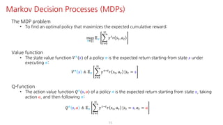
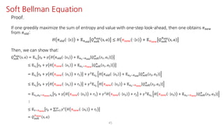
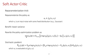
14. A Markov decision process (MDP) is a tuple < 𝑆, 𝐴, 𝑝, 𝑟, 𝛾 >, consisting of
• 𝑆: set of states (state space)
e.g., 𝑆 = 1, … , 𝑛 (discrete), 𝑆 = ℝ:
(continuous)
• 𝐴: set of actions (action space)
e.g., 𝐴 = 1, … , 𝑚 (discrete), 𝐴 = ℝ<
(continuous)
• 𝑝: state transition probability
𝑝 𝑠= 𝑠, 𝑎 ≜ Prob 𝑠"?@ = 𝑠= 𝑠" = 𝑠, 𝑎" = 𝑎 d
• 𝑟: reward function
𝑟 𝑠", 𝑎" = 𝑟"d
• 𝛾 ∈ (0,1]: discount factor
14
Markov Decision Processes (MDPs)

15. The MDP problem
• To find an optimal policy that maximizes the expected cumulative reward:
max
F∈∏
𝔼F I
"JK
L
𝛾" 𝑟 𝑠", 𝑎"
Value function
• The state value function 𝑉F
(𝑠) of a policy 𝜋 is the expected return starting from state 𝑠 under
executing 𝜋:
𝑉F
𝑠 ≜ 𝔼F I
NJ"
L
𝛾NO"
𝑟 𝑠N, 𝑎N |𝑠" = 𝑠
Q-function
• The action value function 𝑄F(𝑠, 𝑎) of a policy 𝜋 is the expected return starting from state 𝑠, taking
action 𝑎, and then following 𝜋:
𝑄F
𝑠, 𝑎 ≜ 𝔼F I
NJ"
L
𝛾NO"
𝑟 𝑠N, 𝑎N |𝑠" = 𝑠, 𝑎" = 𝑎
15
Markov Decision Processes (MDPs)

16. The MDP problem
• To find an optimal policy that maximizes the expected cumulative reward:
max
F∈∏
𝔼F I
"JK
L
𝛾"
𝑟 𝑠", 𝑎"
Optimal value function
• The optimal value function 𝑉∗(𝑠) is the maximum value function over all policies:
𝑉∗ 𝑠 ≜ max
F∈∏
𝑉F 𝑠 = max
F∈∏
𝔼F I
"JK
L
𝛾" 𝑟 𝑠", 𝑎" |𝑠" = 𝑠
Optimal Q-function
• The optimal Q-function 𝑄∗(𝑠, 𝑎) is the maximum Q-function over all policies:
𝑄∗ 𝑠, 𝑎 ≜ max
F∈∏
𝑄F 𝑠, 𝑎
16
Markov Decision Processes (MDPs)

17. Bellman expectation equation for 𝑉F
• The value function 𝑉F is the unique solution to the following Bellman equation:
𝑉F 𝑠 = 𝔼 𝑟 𝑠", 𝑎" + 𝛾𝑉F 𝑠"?@ |𝑠" = 𝑠
= I
S∈T
𝜋(𝑎|𝑠) 𝑟 𝑠, 𝑎 + 𝛾 I
UV∈W
𝑝 𝑠=
𝑠, 𝑎 𝑉F
𝑠=
= I
S∈T
𝜋(𝑎|𝑠)𝑄F
𝑠, 𝑎
• In operator form
𝑉F = 𝑇𝑉F
Bellman expectation equation for 𝑄F
• The Q-function 𝑄F satisfies:
𝑄F 𝑠, 𝑎 = 𝔼 𝑟 𝑠", 𝑎" + 𝛾𝑉F 𝑠"?@ |𝑠" = 𝑠, 𝑎" = 𝑎
= 𝑟 𝑠, 𝑎 + 𝛾 I
UV∈W
𝑝(𝑠=|𝑠, 𝑎)𝑉F 𝑠=
= 𝑟 𝑠, 𝑎 + 𝛾 I
UV∈W
𝑝 𝑠=
𝑠, 𝑎 I
SV∈T
𝜋 𝑎=
𝑠=
𝑄F
𝑠=
, 𝑎=
17
Bellman Equation

18. Bellman optimality equation for 𝑉∗
• The optimal value function 𝑉∗
must satisfies the self-consistency condition given by the Bellman
equation for 𝑉F:
𝑉∗ 𝑠 = max
SY∈T
𝔼 𝑟 𝑠", 𝑎" + 𝛾𝑉∗ 𝑠"?@ |𝑠" = 𝑠
= max
S∈T
𝑟 𝑠, 𝑎 + 𝛾 I
UV∈W
𝑝(𝑠=|𝑠, 𝑎)𝑉∗ 𝑠= = max
S∈T
𝑄∗ 𝑠, 𝑎
• In operator form
𝑉∗
= 𝑇𝑉∗
Bellman optimality equation for 𝑄∗
• The optimal Q-function 𝑄∗ satisfies:
𝑄∗
𝑠, 𝑎 = 𝔼 𝑟 𝑠", 𝑎" + 𝛾𝑉∗
𝑠"?@ |𝑠" = 𝑠, 𝑎" = 𝑎
= 𝑟 𝑠, 𝑎 + 𝛾 I
UV∈W
𝑝(𝑠=|𝑠, 𝑎)𝑉∗ 𝑠=
= 𝑟 𝑠, 𝑎 + 𝛾 I
UV∈W
𝑝(𝑠=|𝑠, 𝑎) max
SV∈T
𝑄∗ 𝑠=, 𝑎=
18
Bellman Equation

19. The MDP problem
• To find an optimal policy that maximizes the expected cumulative reward:
max
F∈∏
𝔼F I
"JK
L
𝛾" 𝑟 𝑠", 𝑎"
Known model:
• Policy iteration
• Value iteration
Unknown model:
• Temporal-difference learning
• Q-learning
19
Bellman Equation

20. Policy Iteration
Initialize a policy 𝜋K;
1. (Policy Evaluation) Compute the value 𝑉F[ of 𝜋
by solving the Bellman equation 𝑉F[ = 𝑇F[ 𝑉F[;
2. (Policy Improvement) Update the policy to 𝜋?@ so that
𝜋?@(𝑠) ∈ arg max
S
{𝑟 𝑠, 𝑎 + 𝛾 I
UV∈W
𝑝 𝑠= 𝑠, 𝑎 𝑉F[ 𝑠= }
3. Set 𝑘 ← 𝑘 + 1; Repeat until convergence;
• Converged policy is optimal!
• Q) Can we do something even simpler?
20
Bellman Equation

21. Value Iteration
Initialize a value function 𝑉K;
1. Update the value function by
𝑉?@ ← 𝑇𝑉;
2. Set 𝑘 ← 𝑘 + 1; Repeat until convergence;
• Converged value function is optimal!
21
Bellman Equation

22. Common issue: exploration
• Is there a value of exploring unknown regions of the environment?
• Which action should we try to explore unknown regions of the environment?
22
Exploration methods

23. How can we algorithmically solve this issue in exploration vs exploitation?
1. 𝜖-Greedy
2. Optimism in the face of uncertainty
3. Thompson (posterior) sampling
4. Noisy networks
5. Information theoretic exploration
23
Exploration methods

24. Method 1: 𝜖-Greedy
Idea:
• Choose a greedy action (arg max 𝑄F(𝑠, 𝑎)) with probability (1 − 𝜖)
• Choose a random action with probability 𝜖
Advantages:
1. Very simple
2. Light computation
Disadvantages:
1. Fine tuning 𝜖
2. Not quite systematic: No focus on unexplored regions
3. Inefficient
24
Exploration methods

25. Method 2: Optimism in the face of uncertainty (OFU)
Idea:
1. Construct a confidence set for MDP parameters using collected samples
2. Choose MDP parameters that give the highest rewards
3. Construct an optimal policy of the optimistically chosen MDP
Advantages:
1. Regret optimal
2. Systematic: More focus on unexplored regions
Disadvantages:
1. Complicated
2. Computation intensive
25
Exploration methods

26. Method 3: Thompson (posterior) sampling
Idea:
1. Sample MDP parameters from posterior distribution
2. Construct an optimal policy of the sampled MDP parameters
3. Update the posterior distribution
Advantages:
1. Regret optimal
2. Systematic: More focus on unexplored regions
Disadvantages:
1. Somewhat complicated
26
Exploration methods

27. Method 4: Noisy networks
Idea:
• Inject noise to the weights of Neural Network
Advantages:
1. Simple
2. Good empirical performance
Disadvantages:
1. Not systematic: No focus on unexplored regions
27
Exploration methods

28. Method 5: Information theoretic exploration
Idea:
• Use high entropy policy to explore more
Advantages:
1. Simple
2. Good empirical performance
Disadvantages:
1. More theoretic analyses needed
28
Exploration methods

29. What is entropy?
• Average rate at which information is produced by a stochastic source of data:
𝐻 𝑝 ≜ − I
e
𝑝e log 𝑝e = 𝔼 − log 𝑝e
• More generally, entropy refers to disorder
29
Maximum Entropy Reinforcement Learning

30. What’s the benefit of high entropy policy?
• Entropy of policy:
𝐻 𝜋(⋅ |𝑠) ≜ − I
S
𝜋(𝑎|𝑠) log 𝜋(𝑎|𝑠) = 𝔼S~F(⋅|U) − log 𝜋(𝑎|𝑠)
• Higher disorder in policy 𝜋
• Try new risky behaviors: Potentially explore unexplored regions
30
Maximum Entropy Reinforcement Learning

31. Maximum entropy stochastic control
Standard MDP problem:
max
F
𝔼F I
"
𝛾" 𝑟(𝑠", 𝑎")
Maximum entropy MDP problem:
max
F
𝔼F I
"
𝛾" 𝑟 𝑠", 𝑎" + 𝐻 𝜋" ⋅ 𝑠"
31
Soft MDPs

32. Theorem 1 (Soft value functions and Optimal policy)
Soft Q-function:
𝑄ijkl
F
𝑠", 𝑎" ≜ 𝑟 𝑠", 𝑎" + 𝔼F I
mJ@
L
𝛾m 𝑟 𝑠"?m, 𝑎"?m + 𝐻 𝜋 ⋅ 𝑠"?m
Soft value function:
𝑉ijkl
F
𝑠" ≜ log n exp 𝑄ijkl
F
𝑠", 𝑎 𝑑𝑎
Optimal value functions:
𝑄ijkl
∗
𝑠", 𝑎" ≜ max
F
𝑄ijkl
F
𝑠", 𝑎"
𝑉ijkl
∗
𝑠" ≜ log n exp 𝑄ijkl
∗
𝑠", 𝑎 𝑑𝑎
32
Soft Bellman Equation

33. Proof.
Maximum entropy MDP problem:
max
F
𝔼F I
"
𝛾"
𝑟 𝑠", 𝑎" + 𝐻 𝜋" ⋅ 𝑠"
Soft value function:
𝑉ijkl
F
𝑠 = 𝔼F I
NJ"
𝛾NO" 𝑟 𝑠N, 𝑎N − log 𝜋 𝑎N 𝑠N |𝑠" = 𝑠
= 𝔼F 𝑟 𝑠", 𝑎" − log 𝜋 𝑎" 𝑠" + 𝛾𝑉ijkl
F
𝑠"?@ |𝑠" = 𝑠
Soft Q-function:
𝑄ijkl
F
s, 𝑎 = 𝔼F I
NJ"
𝛾NO"
𝑟 𝑠N, 𝑎N − log 𝜋 𝑎N 𝑠N |𝑠" = 𝑠, 𝑎" = 𝑎
= 𝔼F 𝑟 𝑠", 𝑎" + 𝛾𝑉ijkl
F
𝑠"?@ |𝑠" = 𝑠, 𝑎" = 𝑎
33
Soft Bellman Equation
note that 𝑄ijkl
F
s, 𝑎 is the same with the original form

34. Proof.
Soft value function:
𝑉ijkl
F
𝑠 = 𝔼F I
NJ"
𝛾NO" 𝑟 𝑠N, 𝑎N − log 𝜋 𝑎N 𝑠N |𝑠" = 𝑠
= 𝔼F 𝑟 𝑠", 𝑎" − log 𝜋 𝑎" 𝑠" + 𝛾𝑉ijkl
F
𝑠"?@ |𝑠" = 𝑠
Soft Q-function:
𝑄ijkl
F
s, 𝑎 = 𝔼F I
NJ"
𝛾NO"
𝑟 𝑠N, 𝑎N − log 𝜋 𝑎N 𝑠N |𝑠" = 𝑠, 𝑎" = 𝑎
= 𝔼F 𝑟 𝑠", 𝑎" + 𝛾𝑉ijkl
F
𝑠"?@ |𝑠" = 𝑠, 𝑎" = 𝑎
Soft value function (rewrite):
𝑉ijkl
F
𝑠 = 𝔼F 𝑟 𝑠", 𝑎" − log 𝜋 𝑎" 𝑠" + 𝛾𝑉ijkl
F
𝑠"?@ |𝑠" = 𝑠
= 𝔼F 𝑄ijkl
F
𝑠", 𝑎" − log 𝜋 𝑎" 𝑠" |𝑠" = 𝑠
34
Soft Bellman Equation

35. Proof.
Given a policy 𝜋jst, define a new policy 𝜋uvw as:
𝜋uvw 𝑎 𝑠 ∝ exp 𝑄ijkl
Fyz{
s, 𝑎
𝜋uvw 𝑎 𝑠 =
exp(𝑄ijkl
Fyz{
s, 𝑎 )
∫ exp(𝑄ijkl
Fyz{
s, 𝑎= ) 𝑑𝑎=
= softmax
S∈T
𝑄ijkl
Fyz{
s, 𝑎
= exp(𝑄ijkl
Fyz{
s, 𝑎 − 𝑉ijkl
Fyz{
𝑠 ) = exp(𝐴ijkl
Fyz{
s, 𝑎 )
Substitute 𝜋uvw 𝑎 𝑠 into 𝑉ijkl
F
𝑠 :
𝑉ijkl
F
𝑠 = 𝔼S~F 𝑄ijkl
F
s, 𝑎 − log
exp 𝑄ijkl
F
s, 𝑎
∫ exp 𝑄ijkl
F
s, 𝑎= 𝑑𝑎=
= 𝔼S~F 𝑄ijkl
F
s, 𝑎 − log exp 𝑄ijkl
F
s, 𝑎 + log n exp 𝑄ijkl
F
s, 𝑎=
𝑑𝑎=
35
Soft Bellman Equation

36. Proof.
Substitute 𝜋uvw 𝑎 𝑠 into 𝑉ijkl
F
𝑠 :
𝑉ijkl
F
𝑠 = 𝔼S~F 𝑄ijkl
F
s, 𝑎 − log exp 𝑄ijkl
F
s, 𝑎 + log n exp 𝑄ijkl
F
s, 𝑎=
𝑑𝑎=
= 𝔼S~F log n exp 𝑄ijkl
F
s, 𝑎=
𝑑𝑎=
= log n exp 𝑄ijkl
F
s, 𝑎= 𝑑𝑎=
∴ 𝑉ijkl
F
𝑠 = log n exp 𝑄ijkl
F
s, 𝑎 𝑑𝑎
36
Soft Bellman Equation
independent from 𝑎

37. Theorem 1 (Soft value functions and Optimal policy)
Soft Q-function:
𝑄ijkl
F
𝑠", 𝑎" ≜ 𝑟 𝑠", 𝑎" + 𝔼F I
mJ@
L
𝛾m 𝑟 𝑠"?m, 𝑎"?m + 𝐻 𝜋 ⋅ 𝑠"?m
Soft value function:
𝑉ijkl
F
𝑠" ≜ log n exp 𝑄ijkl
F
𝑠", 𝑎 𝑑𝑎
Optimal value functions:
𝑄ijkl
∗
𝑠", 𝑎" ≜ max
F
𝑄ijkl
F
𝑠", 𝑎"
𝑉ijkl
∗
𝑠" ≜ log n exp 𝑄ijkl
∗
𝑠", 𝑎 𝑑𝑎
37
Soft Bellman Equation

38. Theorem 2 (Soft policy improvement theorem)
Given a policy 𝜋jst, define a new policy 𝜋uvw as:
𝜋uvw 𝑎 𝑠 ∝ exp 𝑄ijkl
Fyz{
s, 𝑎
Assume that throughout our computation, 𝑄 is bounded and ∫ exp 𝑄 𝑠, 𝑎 𝑑𝑎 is bounded for any 𝑠 (for
both 𝜋jst and 𝜋uvw).
Then,
𝑄ijkl
F€•‚
s, 𝑎 ≥ 𝑄ijkl
Fyz{
s, 𝑎 ∀𝑠, 𝑎
à Monotonic policy improvement
38
Soft Bellman Equation

39. 39
Soft Bellman Equation
Proof.
If one greedily maximize the sum of entropy and value with one-step look-ahead, then one obtains 𝜋uvw
from 𝜋jst:
𝐻 𝜋jst ⋅ 𝑠 + 𝔼Fyz{
𝑄ijkl
Fyz{
s, 𝑎 ≤ 𝐻 𝜋uvw ⋅ 𝑠 + 𝔼F€•‚
𝑄ijkl
Fyz{
s, 𝑎
Example
𝜋(𝑎|𝑠)
𝑟(𝑠, 𝑎)
𝑠K
𝑠@
𝑠†
𝑠‡
𝑠ˆ
𝜋jst
0.5
0.5
0.5
0.5
+2
+4+1
+1
𝑠•
𝑠Ž
0.5
+3
0.5
+1

40. 40
Soft Bellman Equation
Proof.
If one greedily maximize the sum of entropy and value with one-step look-ahead, then one obtains 𝜋uvw
from 𝜋jst:
𝐻 𝜋jst ⋅ 𝑠 + 𝔼Fyz{
𝑄ijkl
Fyz{
s, 𝑎 ≤ 𝐻 𝜋uvw ⋅ 𝑠 + 𝔼F€•‚
𝑄ijkl
Fyz{
s, 𝑎
Example
𝑠K
𝑠@
𝑠†
𝑠‡
𝑠ˆ
𝜋jst
0.5
0.5
0.5
0.5
+2
+4+1
+1
𝑠•
𝑠Ž
0.5
+3
0.5
+1
𝑄ijkl
Fyz{
left = ?
𝑄ijkl
Fyz{
right = ?
𝑄ijkl
Fyz{
left = ?
𝑄ijkl
Fyz{
right = ?
𝑄ijkl
Fyz{
left = ?
𝑄ijkl
Fyz{
right =?
Soft Q-function:
𝑄ijkl
F
𝑠, 𝑎 ≜ 𝑟 𝑠", 𝑎" + 𝔼F I
mJ@
L
𝛾m
𝑟 𝑠"?m, 𝑎"?m + 𝐻 𝜋 ⋅ 𝑠"?m
= 𝑟 𝑠, 𝑎 + 𝛾𝑝 𝑠=
𝑠, 𝑎 𝑉ijkl
F
𝑠=
Soft value function:
𝑉ijkl
F
𝑠 = I
S
𝜋 𝑎 𝑠 𝑄ijkl
F
s, 𝑎 − log 𝜋 𝑎 𝑠
Entropy of policy:
𝐻 𝜋(⋅ |𝑠) ≜ − I
S
𝜋(𝑎|𝑠) log 𝜋(𝑎|𝑠)

41. 41
Soft Bellman Equation
Proof.
If one greedily maximize the sum of entropy and value with one-step look-ahead, then one obtains 𝜋uvw
from 𝜋jst:
𝐻 𝜋jst ⋅ 𝑠 + 𝔼Fyz{
𝑄ijkl
Fyz{
s, 𝑎 ≤ 𝐻 𝜋uvw ⋅ 𝑠 + 𝔼F€•‚
𝑄ijkl
Fyz{
s, 𝑎
Example
𝑠K
𝑠@
𝑠†
𝑠‡
𝑠ˆ
𝜋jst (suppose γ = 1, 𝑝 𝑠=
𝑠, 𝑎 = 1)
0.5
0.5
0.5
0.5
+2
+4+1
+1
𝑠•
𝑠Ž
0.5
+3
0.5
+1
𝑄ijkl
Fyz{
left = 2
𝑄ijkl
Fyz{
right = 4
𝑄ijkl
Fyz{
left = 3
𝑄ijkl
Fyz{
right = 1
𝑄ijkl
Fyz{
left = 4.3
𝑄ijkl
Fyz{
right = 3.3
Soft Q-function:
𝑄ijkl
F
𝑠, 𝑎 ≜ 𝑟 𝑠", 𝑎" + 𝔼F I
mJ@
L
𝛾m
𝑟 𝑠"?m, 𝑎"?m + 𝐻 𝜋 ⋅ 𝑠"?m
= 𝑟 𝑠, 𝑎 + 𝛾𝑝 𝑠=
𝑠, 𝑎 𝑉ijkl
F
𝑠=
Soft value function:
𝑉ijkl
F
𝑠 = I
S
𝜋 𝑎 𝑠 𝑄ijkl
F
s, 𝑎 − log 𝜋 𝑎 𝑠
Entropy of policy:
𝐻 𝜋(⋅ |𝑠) ≜ − I
S
𝜋(𝑎|𝑠) log 𝜋(𝑎|𝑠)

42. 42
Soft Bellman Equation
Proof.
If one greedily maximize the sum of entropy and value with one-step look-ahead, then one obtains 𝜋uvw
from 𝜋jst:
𝐻 𝜋jst ⋅ 𝑠 + 𝔼Fyz{
𝑄ijkl
Fyz{
s, 𝑎 ≤ 𝐻 𝜋uvw ⋅ 𝑠 + 𝔼F€•‚
𝑄ijkl
Fyz{
s, 𝑎
Example
𝑠K
𝑠@
𝑠†
𝑠‡
𝑠ˆ
𝜋jst
0.5
0.5
0.5
0.5
+2
+4+1
+1
𝑠•
𝑠Ž
0.5
+3
0.5
+1
A new policy 𝜋uvw:
𝜋uvw 𝑎 𝑠 ∝ exp 𝑄ijkl
Fyz{
s, 𝑎
𝜋uvw 𝑎 𝑠 =
exp(𝑄ijkl
Fyz{
s, 𝑎 )
∑SV exp(𝑄ijkl
Fyz{
s, 𝑎= )
= softmax
S∈T
𝑄ijkl
Fyz{
s, 𝑎
= exp(𝑄ijkl
Fyz{
s, 𝑎 − 𝑉ijkl
Fyz{
𝑠 )
𝑄ijkl
Fyz{
left = 2
𝑄ijkl
Fyz{
right = 4
𝑄ijkl
Fyz{
left = 3
𝑄ijkl
Fyz{
right = 1
𝑄ijkl
Fyz{
left = 4.3
𝑄ijkl
Fyz{
right = 3.3

43. 43
Soft Bellman Equation
Proof.
If one greedily maximize the sum of entropy and value with one-step look-ahead, then one obtains 𝜋uvw
from 𝜋jst:
𝐻 𝜋jst ⋅ 𝑠 + 𝔼Fyz{
𝑄ijkl
Fyz{
s, 𝑎 ≤ 𝐻 𝜋uvw ⋅ 𝑠 + 𝔼F€•‚
𝑄ijkl
Fyz{
s, 𝑎
Example
𝑠K
𝑠@
𝑠†
𝑠‡
𝑠ˆ
𝜋jst
0.5
0.5
0.5
0.5
+2
+4+1
+1
𝑠•
𝑠Ž
0.5
+3
0.5
+1
𝑄ijkl
Fyz{
left = 2
𝑄ijkl
Fyz{
right = 4
𝑄ijkl
Fyz{
left = 3
𝑄ijkl
Fyz{
right = 1
𝑄ijkl
Fyz{
left = 4.3
𝑄ijkl
Fyz{
right = 3.3
𝑠K
𝑠@
𝑠†
𝑠‡
𝑠ˆ
𝜋uvw 𝜋uvw 𝑎 𝑠 =
v•– —˜y™š
›yz{
i,S
∑
œV v•– —˜y™š
›yz{ i,SV
0.73
0.27
0.12
0.88
+2
+4+1
+1
𝑠•
𝑠Ž
0.88
+3
0.12
+1

44. 44
Soft Bellman Equation
Proof.
If one greedily maximize the sum of entropy and value with one-step look-ahead, then one obtains 𝜋uvw
from 𝜋jst:
𝐻 𝜋jst ⋅ 𝑠 + 𝔼Fyz{
𝑄ijkl
Fyz{
s, 𝑎 ≤ 𝐻 𝜋uvw ⋅ 𝑠 + 𝔼F€•‚
𝑄ijkl
Fyz{
s, 𝑎
So, Substitute 𝑠K, 𝑎K for 𝑠, 𝑎:
𝐻 𝜋jst ⋅ 𝑠K + 𝔼Fyz{
𝑄ijkl
Fyz{
𝑠K, 𝑎K ≤ 𝐻 𝜋uvw ⋅ 𝑠K + 𝔼F€•‚
𝑄ijkl
Fyz{
𝑠K, 𝑎K
0.3 + 3.8 ≤ 0.25 + 4.03
4.1 ≤ 4.28

45. 45
Soft Bellman Equation
Proof.
If one greedily maximize the sum of entropy and value with one-step look-ahead, then one obtains 𝜋uvw
from 𝜋jst:
𝐻 𝜋jst ⋅ 𝑠 + 𝔼Fyz{
𝑄ijkl
Fyz{
s, 𝑎 ≤ 𝐻 𝜋uvw ⋅ 𝑠 + 𝔼F€•‚
𝑄ijkl
Fyz{
s, 𝑎
Then, we can show that:
𝑄ijkl
Fyz{
s, 𝑎 = 𝔼UŸ
𝑟K + 𝛾 𝐻 𝜋jst ⋅ 𝑠@ + 𝔼SŸ~Fyz{
𝑄ijkl
F
𝑠@, 𝑎@
≤ 𝔼UŸ
𝑟K + 𝛾 𝐻 𝜋uvw ⋅ 𝑠@ + 𝔼SŸ~F€•‚
𝑄ijkl
F
𝑠@, 𝑎@
= 𝔼UŸ
𝑟K + 𝛾 𝐻 𝜋uvw ⋅ 𝑠@ + 𝑟@ + 𝛾† 𝔼U 𝐻 𝜋jst ⋅ 𝑠† + 𝔼S ~Fyz{
𝑄ijkl
F
𝑠†, 𝑎†
≤ 𝔼UŸ
𝑟K + 𝛾 𝐻 𝜋uvw ⋅ 𝑠@ + 𝑟@ + 𝛾† 𝔼U 𝐻 𝜋uvw ⋅ 𝑠† + 𝔼S ~F€•‚
𝑄ijkl
F
𝑠†, 𝑎†
= 𝔼UŸ,S ~F€•‚,U 𝑟K + 𝛾 𝐻 𝜋uvw ⋅ 𝑠@ + 𝑟@ + 𝛾† 𝐻 𝜋uvw ⋅ 𝑠† + 𝑟† + 𝛾‡ 𝔼U¡
𝐻 𝜋uvw ⋅ 𝑠‡ + 𝔼S¡~F€•‚
𝑄ijkl
F
𝑠‡, 𝑎‡
⋮
≤ 𝔼N~F€•‚
𝑟K + ∑"J@
L 𝛾" 𝐻 𝜋uvw ⋅ 𝑠" + 𝑟"
= 𝑄ijkl
F€•‚
s, 𝑎

46. Theorem 2 (Soft policy improvement theorem)
Given a policy 𝜋jst, define a new policy 𝜋uvw as:
𝜋uvw 𝑎 𝑠 ∝ exp 𝑄ijkl
Fyz{
s, 𝑎
Assume that throughout our computation, 𝑄 is bounded and ∫ exp 𝑄 𝑠, 𝑎 𝑑𝑎 is bounded for any 𝑠 (for
both 𝜋jst and 𝜋uvw).
Then,
𝑄ijkl
F€•‚
s, 𝑎 ≥ 𝑄ijkl
Fyz{
s, 𝑎 ∀𝑠, 𝑎
à Monotonic policy improvement
46
Soft Bellman Equation

47. Comparison to standard MDP: Bellman expectation equation
Standard:
𝑄F
𝑠, 𝑎 = 𝔼 𝑟 𝑠", 𝑎" + 𝛾𝑉F
𝑠"?@ |𝑠" = 𝑠, 𝑎" = 𝑎
= 𝑟 𝑠, 𝑎 + 𝛾 ∑UV∈W 𝑝(𝑠=
|𝑠, 𝑎)𝑉F
𝑠=
𝑉F
𝑠 = ∑S∈T 𝜋(𝑎|𝑠)𝑄F
𝑠, 𝑎
Maximum entropy:
𝑄ijkl
F
s, 𝑎 = 𝔼F 𝑟 𝑠", 𝑎" + 𝛾𝑉ijkl
F
𝑠"?@ |𝑠" = 𝑠, 𝑎" = 𝑎
= 𝑟 𝑠, 𝑎 + 𝛾 ∑UV∈W 𝑝(𝑠=|𝑠, 𝑎)𝑉ijkl
F
𝑠=
𝑉ijkl
F
𝑠 = 𝔼F 𝑄ijkl
F
𝑠", 𝑎" − log 𝜋 𝑎" 𝑠" |𝑠" = 𝑠
= log ∫ exp 𝑄ijkl
F
s, 𝑎 𝑑𝑎
Maximum entropy variant:
• Add explicit temperature parameter 𝛼
𝑉ijkl
F
𝑠 = 𝔼F 𝑄ijkl
F
𝑠", 𝑎" − 𝛼 log 𝜋 𝑎" 𝑠" |𝑠" = 𝑠
= 𝛼 log ∫ exp
@
¤
𝑄ijkl
F
s, 𝑎 𝑑𝑎
47
Soft Bellman Equation

48. Comparison to standard MDP: Bellman optimality equation
Standard:
𝑄∗
𝑠, 𝑎 = 𝔼 𝑟 𝑠", 𝑎" + 𝛾𝑉∗
𝑠"?@ |𝑠" = 𝑠, 𝑎" = 𝑎
= 𝑟 𝑠, 𝑎 + 𝛾 ∑UV∈W 𝑝(𝑠=|𝑠, 𝑎)𝑉∗ 𝑠=
𝑉∗ 𝑠 = max
S∈T
𝑄∗ 𝑠, 𝑎
Maximum entropy variant:
𝑄ijkl
∗
s, 𝑎 = 𝔼F 𝑟 𝑠", 𝑎" + 𝛾𝑉ijkl
∗
𝑠"?@ |𝑠" = 𝑠, 𝑎" = 𝑎
= 𝑟 𝑠, 𝑎 + 𝛾 ∑UV∈W 𝑝(𝑠=|𝑠, 𝑎)𝑉ijkl
∗
𝑠=
𝑉ijkl
∗
𝑠 = 𝔼F 𝑄ijkl
∗
𝑠", 𝑎" − 𝛼 log 𝜋 𝑎" 𝑠" |𝑠" = 𝑠
= 𝛼 log ∫ exp
@
¤
𝑄ijkl
∗
s, 𝑎 𝑑𝑎
Connection:
• Note that as 𝛼 → 0, exp
@
¤
𝑄ijkl
∗
s, 𝑎 emphasizes max
S∈T
𝑄∗ 𝑠, 𝑎 :
𝛼 log ∫ exp
@
¤
𝑄ijkl
∗
s, 𝑎 𝑑𝑎 → max
S∈T
𝑄∗ 𝑠, 𝑎 as 𝛼 → 0
48
Soft Bellman Equation

49. Comparison to standard MDP: Policy
Standard:
𝜋uvw 𝑎 𝑠 ∈ arg max
S
𝑄Fyz{ 𝑠, 𝑎
à Deterministic policy
Maximum Entropy:
𝜋uvw 𝑎 𝑠 =
exp
1
𝛼
𝑄ijkl
Fyz{
s, 𝑎
∫ exp
1
𝛼
𝑄ijkl
Fyz{
s, 𝑎= 𝑑𝑎=
= exp
1
𝛼
𝑄ijkl
Fyz{
s, 𝑎 − 𝑉ijkl
Fyz{
𝑠
à Stochastic policy
49
Soft Bellman Equation

50. So, what’s the advantage of maximum entropy?
• Computation:
No maximization involved
• Exploration:
High entropy policy
• Structural similarity:
Can combine it with many RL methods for standard MDP
50
Soft Bellman Equation

51. Idea:
• Maximum entropy + off-policy actor-critic
Advantages:
• Exploration
• Sample efficiency
• Stable convergence
• Little hyperparameter tuning
51
From Soft Policy Iteration to Soft Actor-Critic
Version 1 (Jan 4 2018) Version 2 (Dec 13 2018)

52. Soft policy evaluation
Modified Bellman operator:
𝑇F
𝑄F
𝑠, 𝑎 ≜ 𝑟 𝑠, 𝑎 + 𝛾 I
UV∈W
𝑝(𝑠=
|𝑠, 𝑎)𝑉ijkl
F
𝑠=
where 𝑉F 𝑠 = 𝔼F 𝑄ijkl
F
s, 𝑎 − 𝛼 log 𝜋 𝑎 𝑠
Repeatedly apply 𝑇F
to 𝑄:
𝑄?@ ← 𝑇F 𝑄
• Result: 𝑄 converges to 𝑄F!
52
Soft Policy Iteration

53. Soft policy improvement
If no constraint on policies,
𝜋uvw 𝑎 𝑠 = exp
1
𝛼
𝑄ijkl
Fyz{
s, 𝑎 − 𝑉ijkl
Fyz{
𝑠
When constraint need to be satisfied (i.e., 𝜋 ∈ ∏),
Information projection:
𝜋uvw ⋅ 𝑠 ∈ arg min
FV ⋅ 𝑠 ∈∏
𝐷¨© 𝜋= ⋅ 𝑠 ∥ exp
1
𝛼
𝑄ijkl
Fyz{
s,⋅ − 𝑉ijkl
Fyz{
𝑠
• Result: Monotonic improvement on policy! (𝜋uvw better than 𝜋jst)
53
target policy
Soft Policy Iteration

54. Model-Free version of soft policy iteration: Soft actor-critic
Soft policy iteration: maximum entropy variant of policy iteration
Soft actor-critic (SAC): maximum entropy variant of actor-critic
• Soft critic:
evaluates soft Q-function 𝑄« of policy 𝜋¬
• Soft actor:
improves maximum entropy policy using critic’s evaluation
• Temperature parameter alpha:
automatically adjusts entropy for maximum entropy policy using alpha 𝛼
54
Soft Actor-Critic

55. Soft critic: evaluates soft Q-function 𝑄« of policy 𝜋¬
Idea: DQN + Maximum entropy
• Training soft Q-function:
min
«
𝐽— 𝜃 ≜ 𝔼 UY,SY
1
2
𝑄« 𝑠", 𝑎" − 𝑟 𝑠", 𝑎" + 𝛾𝔼UY¯Ÿ
𝑉«° 𝑠"?@
†
• Stochastic gradient:
±∇« 𝐽— 𝜃 = ∇« 𝑄« 𝑠", 𝑎" × 𝑄« 𝑠", 𝑎" − 𝑟 𝑠", 𝑎" + 𝛾 𝑄«° 𝑠"?@, 𝑎"?@ − 𝛼 log 𝜋¬ 𝑎"?@ 𝑠"?@
55
Soft Actor-Critic
target
sample estimate of 𝔼UY¯Ÿ
𝑉«° 𝑠"?@

56. Soft actor: updates policy using critic’s evaluation
Idea: Policy gradient + Maximum entropy
• Minimizing the expected KL-divergence:
min
¬
𝐷¨© 𝜋¬ ⋅ 𝑠" ∥ exp
1
𝛼
𝑄« 𝑠",⋅ − 𝑉« 𝑠"
which is equivalent to
min
¬
𝐽F 𝜙 ≜ 𝔼UY
𝔼SY~Fµ ⋅ 𝑠"
𝛼 log 𝜋¬ 𝑎" 𝑠" − 𝑄« 𝑠", 𝑎"
56
Soft Actor-Critic
target policy

57. Reparameterization trick
Reparameterize the policy as
𝑎" ≜ 𝑓¬ 𝜖"; 𝑠"
which 𝜖" is an input noise with some fixed distribution (e.g., Gaussian)
Benefit: lower variance
Rewrite the policy optimization problem as
min
¬
𝐽F 𝜙 ≜ 𝔼UY,·Y
𝛼 log 𝜋¬ 𝑓¬ 𝜖"; 𝑠" 𝑠" − 𝑄« 𝑠", 𝑓¬ 𝜖"; 𝑠"
Stochastic gradient:
±∇¬ 𝐽F 𝜙 = ∇¬ 𝛼 log 𝜋¬ 𝑎" 𝑠" + ∇SY
𝛼 log 𝜋¬ 𝑎" 𝑠" − ∇SY
𝑄« 𝑠", 𝑎" ×∇¬ 𝑓¬ 𝜖"; 𝑠"
which 𝑎" is evaluated at 𝑓¬ 𝜖"; 𝑠"
57
Soft Actor-Critic

58. Automating entropy adjustment
Why do we have to do automatic temperature parameter 𝛼 adjustment?
• Choosing the optimal temperature 𝛼"
∗ is non-trivial, and the temperature needs to be tuned for each task.
• Since the entropy 𝐻 𝜋" can vary unpredictably both across tasks and during training as the policy becomes
better, this makes the temperature adjustment particularly difficult.
• Thus, simply forcing the entropy to a fixed value is a poor solution, since the policy should be free to explore
more in regions.
58
Soft Actor-Critic

59. Automating entropy adjustment
Constrained optimization problem suppose 𝛾 = 1 :
max
F¸,…,F¹
𝔼 I
"JK
º
𝑟(𝑠", 𝑎") s. t. 𝐻 𝜋" ≥ 𝐻K ∀𝑡
where 𝐻K is a desired minimum expected entropy threshold
Rewrite the objective as an iterated maximization employing an (approximate) dynamic programming
approach:
max
F¸
𝔼 𝑟 𝑠K, 𝑎K + max
FŸ
𝔼 … + max
F¹
𝔼 𝑟 𝑠º, 𝑎º
Subject to the constraint on entropy
Start from the last time step 𝑇:
max
F¹
𝔼 U¹,S¹ ~¼›
𝑟 𝑠º, 𝑎º
Subject to 𝔼 U¹,S¹ ~¼›
− log 𝜋º 𝑎º 𝑠º − 𝐻K ≥ 0
59
Soft Actor-Critic

60. Automating entropy adjustment
Change the constrained maximization to the dual problem using Lagrangian:
1. Create the following function:
𝑓 𝜋º = ½
𝔼 U¹,S¹ ~¼›
𝑟 𝑠º, 𝑎º , s. t. ℎ(𝜋º) ≥ 0
−∞, otherwise
ℎ 𝜋º = 𝐻 𝜋º − 𝐻K = 𝔼 U¹,S¹ ~¼›
− log 𝜋º 𝑎º 𝑠º − 𝐻K
2. So, rewrite the objective as
max
F¹
𝑓 𝜋º s. t. ℎ 𝜋º ≥ 0
3. Use Lagrange multiplier:
min
¤¹ÁK
𝐿 𝜋º, 𝛼º = 𝑓 𝜋º + 𝛼ºℎ 𝜋º
where 𝛼º is the dual variable
4. Rewrite the objective using Lagrangian as
max
F¹
𝑓 𝜋º = min
¤¹ÁK
max
F¹
𝐿 𝜋º, 𝛼º = min
¤¹ÁK
max
F¹
𝑓 𝜋º + 𝛼ºℎ 𝜋º
60
Soft Actor-Critic

61. Automating entropy adjustment
Change the constrained maximization to the dual problem using Lagrangian:
max
F¹
𝔼 U¹,S¹ ~¼›
𝑟 𝑠º, 𝑎º = max
F¹
𝑓 𝜋º
= min
¤¹ÁK
max
F¹
𝐿 𝜋º, 𝛼º = min
¤¹ÁK
max
F¹
𝑓 𝜋º + 𝛼ºℎ 𝜋º
= min
¤¹ÁK
max
F¹
𝔼 U¹,S¹ ~¼›
𝑟 𝑠º, 𝑎º + 𝛼º 𝔼 U¹,S¹ ~¼›
− log 𝜋º 𝑎º 𝑠º − 𝐻K
= min
¤¹ÁK
max
F¹
𝔼 U¹,S¹ ~¼›
𝑟 𝑠º, 𝑎º − 𝛼º log 𝜋º 𝑎º 𝑠º − 𝛼º 𝐻K
= min
¤¹ÁK
max
F¹
𝔼 U¹,S¹ ~¼›
𝑟 𝑠º, 𝑎º + 𝛼º 𝐻 𝜋º − 𝛼º 𝐻K
We can solve for
• Optimal policy 𝜋º
∗
as
𝜋º
∗ = arg max
F¹
𝔼 U¹,S¹ ~¼›
𝑟 𝑠º, 𝑎º + 𝛼º 𝐻 𝜋º − 𝛼º 𝐻K
• Optimal dual variable 𝛼º
∗
as
𝛼º
∗
= arg min
¤¹ÁK
𝔼 U¹,S¹ ~¼›∗ 𝛼º 𝐻 𝜋º
∗
− 𝛼º 𝐻K
Thus,
max
F¹
𝔼 𝑟 𝑠º, 𝑎º = 𝔼 U¹,S¹ ~¼›∗ 𝑟 𝑠º, 𝑎º + 𝛼º
∗ 𝐻 𝜋º
∗ − 𝛼º
∗ 𝐻K
61
Soft Actor-Critic

62. Automating entropy adjustment
Then, the soft Q-function can be computed as
𝑄ºO@ 𝑠ºO@, 𝑎ºO@ = 𝑟 𝑠ºO@, 𝑎ºO@ + 𝔼 𝑄º 𝑠º, 𝑎º − 𝛼º log 𝜋º 𝑎º 𝑠º
= 𝑟 𝑠ºO@, 𝑎ºO@ + 𝔼 𝑟 𝑠º, 𝑎º + 𝛼º 𝐻 𝜋º
𝑄ºO@
∗
𝑠ºO@, 𝑎ºO@ = 𝑟 𝑠ºO@, 𝑎ºO@ + max
F¹
𝔼 𝑟 𝑠º, 𝑎º + 𝛼º
∗
𝐻(𝜋º
∗
)
Now, given the time step 𝑇 − 1, we have:
max
F¹°Ÿ
𝔼 𝑟 𝑠ºO@, 𝑎ºO@ + max
F¹
𝔼 𝑟 𝑠º, 𝑎º
= max
F¹°Ÿ
𝑄ºO@
∗
𝑠ºO@, 𝑎ºO@ − 𝛼º
∗
𝐻 𝜋º
∗
= min
¤¹°ŸÁK
max
F¹°Ÿ
𝑄ºO@
∗
𝑠ºO@, 𝑎ºO@ − 𝛼º
∗
𝐻 𝜋º
∗
+ 𝛼ºO@ 𝐻 𝜋ºO@ − 𝐻K
= min
¤¹°ŸÁK
max
F¹°Ÿ
𝑄ºO@
∗
𝑠ºO@, 𝑎ºO@ − 𝛼ºO@ 𝐻 𝜋ºO@ − 𝛼ºO@ 𝐻K − 𝛼º
∗
𝐻 𝜋º
∗
62
Soft Actor-Critic

63. Automating entropy adjustment
We can solve for
• Optimal policy 𝜋ºO@
∗
as
𝜋ºO@
∗
= arg max
F¹°Ÿ
𝔼 U¹°Ÿ,S¹°Ÿ ~¼›
𝑄ºO@
∗
𝑠ºO@, 𝑎ºO@ + 𝛼ºO@ 𝐻 𝜋ºO@ − 𝛼ºO@ 𝐻K
• Optimal dual variable 𝛼ºO@
∗
as
𝛼ºO@
∗ = arg min
¤¹°ŸÁK
𝔼 U¹°Ÿ,S¹°Ÿ ~¼›∗ 𝛼ºO@ 𝐻 𝜋ºO@
∗ − 𝛼ºO@ 𝐻K
In this way, we can proceed backwards in time and recursively optimize constrained optimization
problem. Then, we can solve the optimal dual variable 𝛼"
∗
after solving for 𝑄"
∗
and 𝜋"
∗
:
𝛼"
∗
= arg min
¤Y
𝔼SY~FY
∗ −𝛼" log 𝜋"
∗
𝑎" 𝑠" − 𝛼" 𝐻K
63
Soft Actor-Critic

64. Temperature parameter alpha: automatically adjusts entropy for maximum entropy policy
using alpha 𝛼
Idea: Constrained optimization problem + Dual problem
• Minimizing the dual objective by approximating dual gradient descent:
min
¤
𝔼SY~FY
−𝛼 log 𝜋" 𝑎" 𝑠" − 𝛼𝐻K
64
Soft Actor-Critic

65. Putting everything together: Soft Actor-Critic (SAC)
65
Soft Actor-Critic

66. 66
Results
• Soft actor-critic (blue and yellow) performs consistently across all tasks and outperforming both
on-policy and off-policy methods in the most challenging tasks.

67. 67
References
Papers
• T. Haarnoja, et al., “Reinforcement Learning with Deep Energy-Based Policies”, ICML 2017
• T. Haarnoja, et, al., “Soft Actor-Critic: Off-Policy Maximum Entropy Deep Reinforcement Learning
with a Stochastic Actor”, ICML 2018
• T. Haarnoja, et, al., “Soft Actor-Critic Algorithms and Applications”, arXiv preprint 2018
Theoretical analysis
• “Induction of Q-learning, Soft Q-learning, and Sparse Q-learning” written by Sungjoon Choi
• “Reinforcement Learning with Deep Energy-Based Policies” reviewed by Kyungjae Lee
• “Entropy Regularization in Reinforcement Learning (Stochastic Policy)” reviewed by Kyungjae Lee
• Reframing Control as an Inference Problem, CS 294-112: Deep Reinforcement Learning
• Constrained optimization problem and dual problem for SAC with automatically adjusted
temperature (in Korean)

68. 68
Any Questions?

69. 69
Thank You