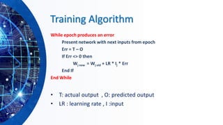
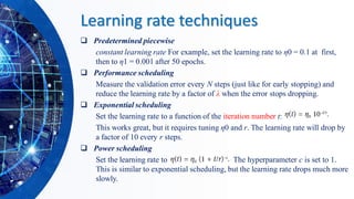
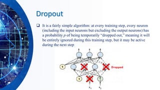
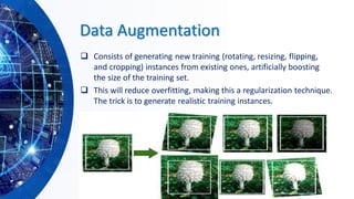
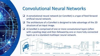
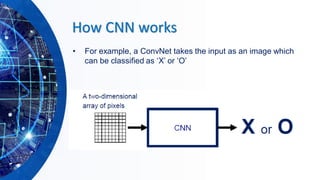
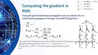
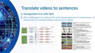
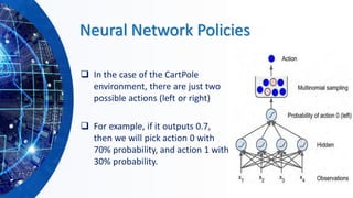
The document provides an overview of machine learning concepts, particularly focusing on artificial neural networks (ANNs) and their various architectures like convolutional neural networks (CNNs) and recurrent neural networks (RNNs). It covers training techniques, activation functions, optimization strategies, and challenges such as vanishing and exploding gradients, as well as solutions like batch normalization and dropout. Overall, it emphasizes the advancements in neural networks and the importance of leveraging existing models through transfer learning.
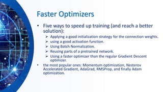
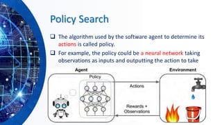
![ConvNet Layers
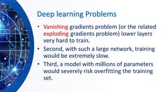
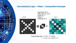
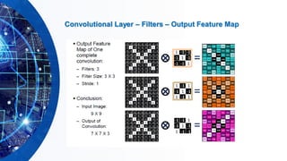
▪CONV layer will compute the output of neurons that are connected
to local regions in the input, each computing a dot product between
their weights and a small region they are connected to in the input
volume.
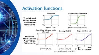
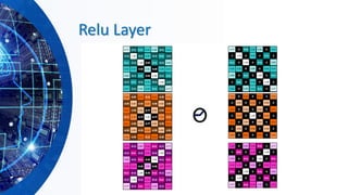
▪RELU layer will apply an elementwise activation function, such as
the max(0,x) thresholding at zero. This leaves the size of the
volume unchanged.
▪POOL layer will perform a down sampling operation along the
spatial dimensions (width, height).
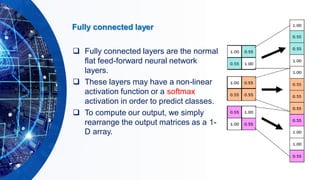
▪FC (i.e. fully-connected) layer will compute the class scores,
resulting in volume of size [1x1xN], where each of the N numbers
correspond to a class score, such as among the N categories.](https://image.slidesharecdn.com/hands-onmachinelearningwithscikit-learnandtensorflowbyahmedyousry-200608190215/85/Hands-on-machine-learning-with-scikit-learn-and-tensor-flow-by-ahmed-yousry-38-320.jpg)
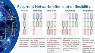
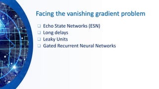
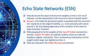
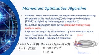
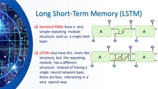
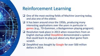
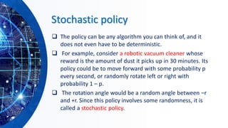
![Gated Recurrent Neural Networks
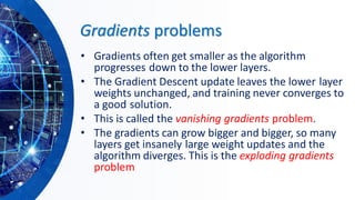
❑ GRNNs are a special kind of RNN, capable of learning long-term
dependencies by having more persistent memory. Two popular
architectures:
➢ Long short-term memory (LSTM) [Hochreiter and Schmidhuber,
1997].
➢ Gated recurrent unit (GRU), [Cho et al., 2014]
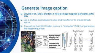
❑ Applications: handwriting recognition (Graves et al., 2009), speech
recognition (Graves et al., 2013; Graves and Jaitly, 2014), handwriting
generation (Graves, 2013), machine translation (Sutskever et al., 2014a),
image to text conversion (captioning) (Kiros et al., 2014b; Vinyals et al.,
2014b; Xu et al., 2015b) and parsing (Vinyals et al., 2014a).](https://image.slidesharecdn.com/hands-onmachinelearningwithscikit-learnandtensorflowbyahmedyousry-200608190215/85/Hands-on-machine-learning-with-scikit-learn-and-tensor-flow-by-ahmed-yousry-64-320.jpg)
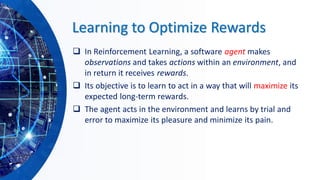
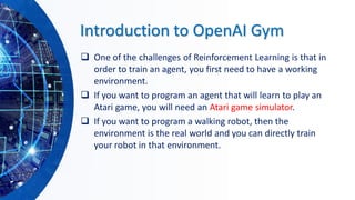
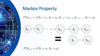
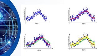
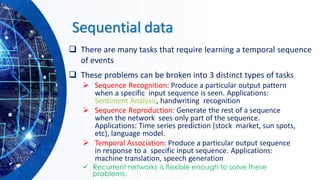
![Utilities of Sequences
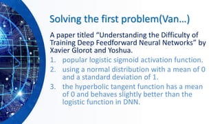
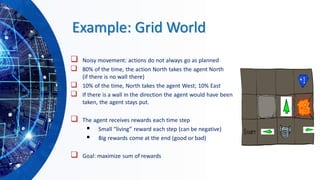
▪ What preferences should an agent have over reward sequences?
▪ More or less?
▪ Now or later?
[1, 2, 2] [2, 3, 4]or
[0, 0, 1] [1, 0, 0]or](https://image.slidesharecdn.com/hands-onmachinelearningwithscikit-learnandtensorflowbyahmedyousry-200608190215/85/Hands-on-machine-learning-with-scikit-learn-and-tensor-flow-by-ahmed-yousry-86-320.jpg)
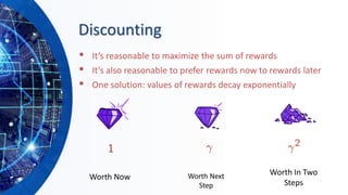
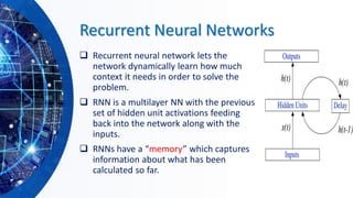
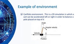
![Discounting
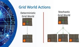
▪ How to discount?
▪ Each time we descend a level, we
multiply in the discount once
▪ Why discount?
▪ Sooner rewards probably do have higher
utility than later rewards
▪ Also helps our algorithms converge
▪ Example: discount of 0.5
▪ U([1,2,3]) = 1*1 + 0.5*2 + 0.25*3
▪ U([1,2,3]) < U([3,2,1])](https://image.slidesharecdn.com/hands-onmachinelearningwithscikit-learnandtensorflowbyahmedyousry-200608190215/85/Hands-on-machine-learning-with-scikit-learn-and-tensor-flow-by-ahmed-yousry-88-320.jpg)


![Deep learning in python ommunic [CNN].pptx](https://cdn.slidesharecdn.com/ss_thumbnails/deeplearninginpythoncnn-251207084743-a5c807e1-thumbnail.jpg?width=640&height=640&fit=bounds)


