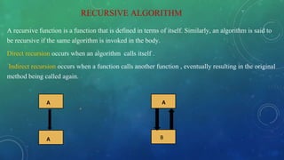
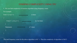
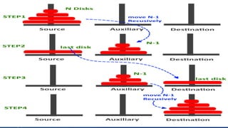
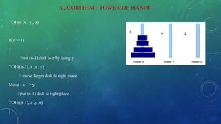
The document discusses the complexity analysis of recursive functions, outlining the definitions and properties of recursive algorithms including direct and indirect recursion. It explains the significance of time and space complexity in both recursive and iterative approaches, emphasizing the use of recurrence relations for analyzing recursive algorithms when frequency counting is insufficient. The document also provides examples, including the Tower of Hanoi, to illustrate the process of establishing and solving recurrence relations for evaluating computational complexity.


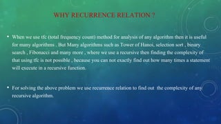


![Expanding:
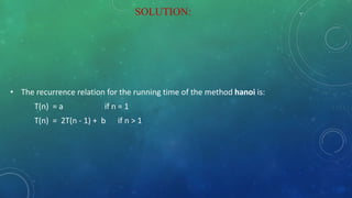
T(1) = a (1)
T(n) = 2T(n – 1) + b if n > 1 (2)
= 2[2T(n – 2) + b] + b = 22 T(n – 2) + 2b + b by substituting T(n – 1) in (2)
= 22 [2T(n – 3) + b] + 2b + b = 23 T(n – 3) + 22b + 2b + b by substituting T(n-2) in (2)
= 23 [2T(n – 4) + b] + 22b + 2b + b = 24 T(n – 4) + 23 b + 22b + 21b + 20b by substituting
T(n – 3) in (2)
= ……
= 2k T(n – k) + b[2k- 1 + 2k– 2 + . . . 21 + 20]
The base case is reached when n – k = 1 k = n – 1, we then have:
Therefore the complexity of Tower of Hanoi is O(2n).](https://image.slidesharecdn.com/22prashijain-200413102924/85/Complexity-Analysis-of-Recursive-Function-17-320.jpg)


![PCC_CS_404_OUCHITYAPRODHAN_17000124029[1].pptx](https://cdn.slidesharecdn.com/ss_thumbnails/pcccs404ouchityaprodhan170001240291-250416041539-b214e64e-thumbnail.jpg?width=640&height=640&fit=bounds)