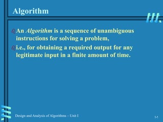
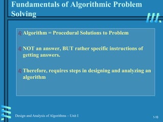
1. An algorithm is a sequence of unambiguous instructions to solve a problem and obtain an output for any valid input in a finite amount of time. Pseudocode is used to describe algorithms using a natural language format.
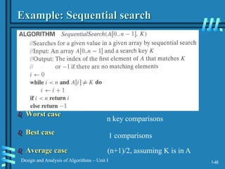
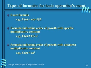
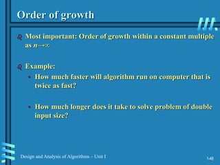
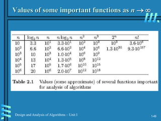
2. Analyzing algorithm efficiency involves determining the theoretical and empirical time complexity by counting the number of basic operations performed relative to the input size. Common measures are best-case, worst-case, average-case, and amortized analysis.
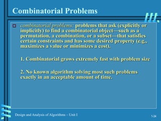
3. Important problem types for algorithms include sorting, searching, string processing, graphs, combinatorics, geometry, and numerical problems. Fundamental algorithms are analyzed for correctness and time/space complexity.

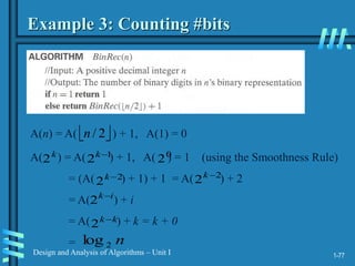
![1-11
Design and Analysis of Algorithms – Unit I
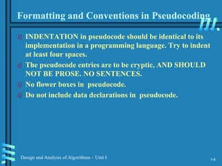
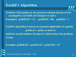
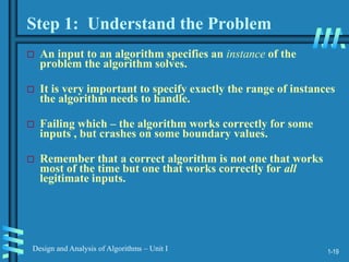
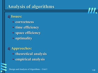
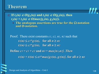
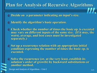
Other methods for gcd(m,n) [cont.]
Middle-school procedure
Step 1 Find the prime factorization of m
Step 2 Find the prime factorization of n
Step 3 Find all the common prime factors
Step 4 Compute the product of all the common prime factors
and return it as gcd(m,n)
Is this an algorithm?](https://image.slidesharecdn.com/analysis-and-design-of-algorithm-230212162018-f2bb9413/85/ANALYSIS-AND-DESIGN-OF-ALGORITHM-ppt-12-320.jpg)
![1-12
Design and Analysis of Algorithms – Unit I
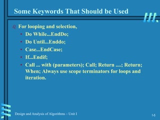
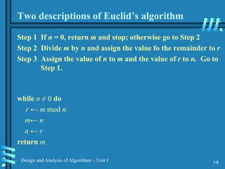
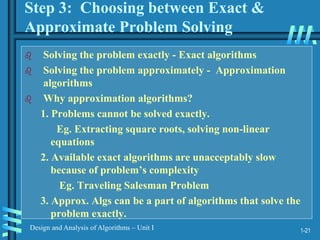
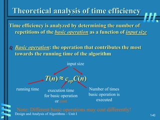
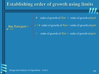
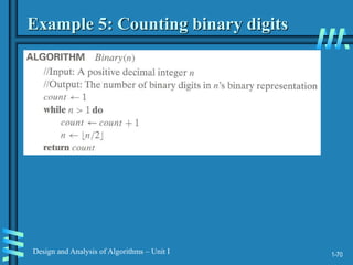
Sieve of Eratosthenes
Input: Integer n ≥ 2
Output: List of primes less than or equal to n
for p ← 2 to n do A[p] ← p
for p ← 2 to n do
if A[p] 0 //p hasn’t been previously eliminated from the list
j ← p* p
while j ≤ n do
A[j] ← 0 //mark element as eliminated
j ← j + p
Example: 2 3 4 5 6 7 8 9 10 11 12 13 14 15 16 17 18 19 20](https://image.slidesharecdn.com/analysis-and-design-of-algorithm-230212162018-f2bb9413/85/ANALYSIS-AND-DESIGN-OF-ALGORITHM-ppt-13-320.jpg)


![1-69
Design and Analysis of Algorithms – Unit I
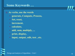
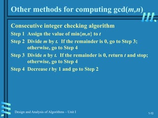
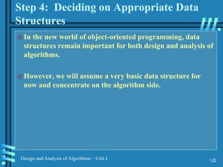
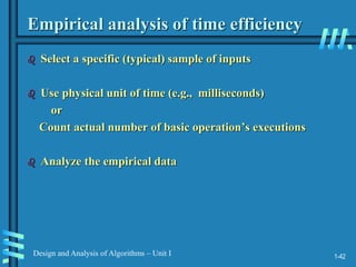
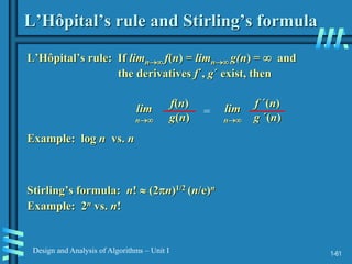
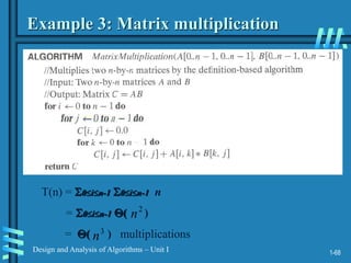
Example 4: Gaussian elimination
Algorithm GaussianElimination(A[0..n-1,0..n])
//Implements Gaussian elimination on an n-by-(n+1) matrix A
for i 0 to n - 2 do
for j i + 1 to n - 1 do
for k i to n do
A[j,k] A[j,k] - A[i,k] A[j,i] / A[i,i]
Find the efficiency class and a constant factor improvement.
for i 0 to n - 2 do
for j i + 1 to n - 1 do
B A[j,i] / A[i,i]
for k i to n do
A[j,k] A[j,k] – A[i,k] * B](https://image.slidesharecdn.com/analysis-and-design-of-algorithm-230212162018-f2bb9413/85/ANALYSIS-AND-DESIGN-OF-ALGORITHM-ppt-70-320.jpg)


![[Make a Copy] Region - Team Name - Project Name.pptx](https://cdn.slidesharecdn.com/ss_thumbnails/makeacopyregion-teamname-projectname-230502014105-e31b8a52-thumbnail.jpg?width=640&height=640&fit=bounds)