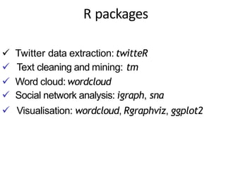
The document presents a project on text mining of Twitter data conducted by students at Birla Institute of Technology, Mesra, Jaipur. It covers the process of extracting tweets, cleaning the text, analyzing word frequency, and creating visualizations such as word clouds, utilizing various R packages for these tasks. Additionally, it provides technical details about authentication, data retrieval, and processing steps involved in text mining using R software.

1. BIRLA INSTITUTE OF TECHNOLOGY
MESRA ,JAIPUR CAMPUS
TOPIC :-TEXT MINING OF TWITTER
PRESENTED BY:
MEGHAJ KUMAR MALLICK(MCA/25017/18)
SAJAN SINGH(MCA/25019/18)
2ND YEAR,3RD SEMESTER

2. OUTLINE
 INTRODUCTION
 Tweets Analysis
Extracting Tweets
Text Cleaning
Frequent Words and Word Cloud
 R Packages
Referencesand OnlineResources

3. TWITTER
Twitter is a microblogging and social networking service on which users post and
interact with messages known as "tweets". Tweets were originally restricted to 140
characters, but on November 7, 2017, this limit was doubled to 280 for all languages
except Chinese, Japanese, and Korean.
Twitter was created in March 2006 by Jack Dorsey, Noah Glass, Biz Stone, and Evan
Williams, launched in July of that year.
 In 2012, more than 100 million users posted 340 million tweets a day, and the
service handled an average of 1.6 billion search queries per day.
In 2013, it was one of the ten most-visited websites and has been described as "the
SMS of the Internet“.
As of 2018, Twitter had more than 321 million monthly active users.

4. PROCESS
1. Extract tweets and followers from the Twitter website with R
and the twitteRpackage
2. With the tm package, clean text by removing punctuations,
numbers, hyperlinks and stop words, followed by stemming
and stem completion
3. Build aterm-document matrix
4. Analyse following/followed and retweeting relationships with
the igraphpackage

5. Retrieving Text from Twitter
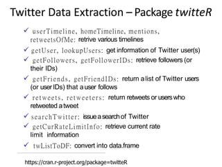
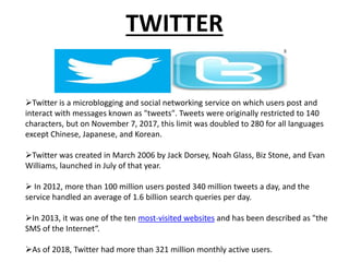
 Tweets are extracted from Twitter with the code below using userTimeline() in package
twitteR [Gentry, 2012]. Package twitteR depends on package RCurl [Lang, 2012a], which is
available at http://www.stats.ox.ac.uk/ pub/RWin/bin/windows/contrib/.
 Another way to retrieve text from Twitter is using package XML [Lang, 2012b], and an
example on that is given at http://heuristically.wordpress.com/ 2011/04/08/text-data-mining-
twitter-r/. For readers who have no access to Twitter, the tweets data “rdmTweets.RData” can
be downloaded at http://www.rdatamining.com/data.
Note that the Twitter API requires authentication since March 2013. Before running the code
below, please complete authentication by following instructions in “Section 3: Authentication
with OAuth” in the twitteR vignettes (http://cran.r-project.org/web/packages/twitteR/
vignettes/twitteR.pdf).

6. Retrieve Tweets
## Option 1: retrieve tweets from Twitter
l i b r a r y (twitteR)
library(ROAuth)
## Twitter authentication
setup_twitter_oauth(consumer_key, consumer_secret, access_token,
access_secret)
## 3200 i s the maximum to retrieve
tweets <- userTimeline("RDataMining", n = 3200)
## Option 2: download @RDataMining tweets from RDataMining.com
u r l <- "http://www.rdatamining.com/data/RDataMining-Tweets-20160212.rds
download .file(url, d e s t f i l e = "./data/RDataMining-Tweets-20160212.rds")
## load tweets into R
tweets <- readRDS("./data/RDataMining-Tweets-20160212.rds")
Twitter Authentication with OAuth:
Section 3 of http://geoffjentry.hexdump.org/twitteR.pdf

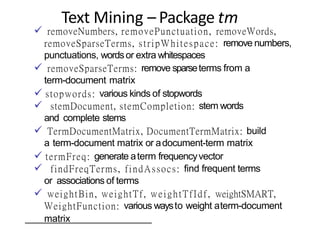
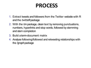
7. (n.tweet <- length(tweets))
## [ 1] 448
# convert tweets to a data frame
tweets.df <- twListToDF(tweets)
# tweet #190
tweets.df[ 190, c ( " i d " , "created" , "screenName", "replyToSN",
"favoriteCount", "retweetCount", "longitude", " l a t i t u d e " , " t e x t " ) ]
## i d created screenName r e . . .
## 190 362866933894352898 2013-08-01 09:26:33 RDataMining . . .
favoriteCount retweetCount longitude l a t i t u d e
9 9 NA NA
##
## 190
## . . .
## 190 The RReference Card f or Data Mining now provides l i n . . .
# print tweet #190 and make t e x t f i t for slide width
writeLines(strwrap(tweets.df$text[190], 60))
## The R Reference Card f or Data Mining now provides l i nks t o ##
packages on CRAN. Packages f or MapReduce and Hadoop added. ##
http://t.co/RrFypol8kw

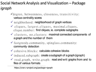
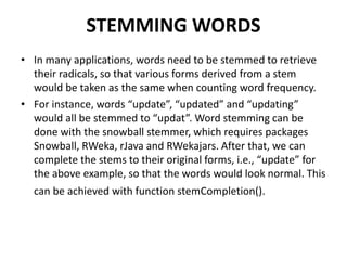
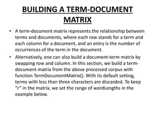
8. TRANSFORMING TEXT
• The tweets are first converted to a data frame and then to a
corpus, which is a collection of text documents. After that, the
corpus can be processed with functions provided in package
tm [Feinerer, 2012].
• # convert tweets to a data frame
• df <- do.call("rbind", lapply(rdmTweets, as.data.frame))
• dim(df)
• [1] 154 10 > library(tm)
• # build a corpus, and specify the source to be character
vectors > myCorpus <- Corpus(VectorSource(df$text))

9. Text Cleaning
library(tm)
# build a corpus, and specify the source to be character vectors
myCorpus <- Corpus(VectorSource(tweets.df$text))
# convert to lower case
myCorpus <- tm_map(myCorpus, content_transformer(tolower))
# remove URLs
removeURL <- function(x) gsub("ht t p[ ^[ : s pace: ]] *" , " " , x)
myCorpus <- tm_map(myCorpus, content_transformer(removeURL))
# remove anything other than English l e t t e r s or space
removeNumPunct <- function(x) gsub("[ ^[ :al p ha :][ :s pace:]] *" , " " , x)
myCorpus <- tm_map(myCorpus, content_transformer(removeNumPunct))
# remove stopwords
myStopwords <- c(setdiff(stopwords('english'), c ( " r " , " b i g " ) ) ,
"use", "s e e " , "used", " v i a " , "amp")
myCorpus <- tm_map(myCorpus, removeWords, myStopwords)
# remove extra whitespace
myCorpus <- tm_map(myCorpus, stripWhitespace)
# keep a copy for stem completion later
myCorpusCopy <- myCorpus

10. STEMMING WORDS
• In many applications, words need to be stemmed to retrieve
their radicals, so that various forms derived from a stem
would be taken as the same when counting word frequency.
• For instance, words “update”, “updated” and “updating”
would all be stemmed to “updat”. Word stemming can be
done with the snowball stemmer, which requires packages
Snowball, RWeka, rJava and RWekajars. After that, we can
complete the stems to their original forms, i.e., “update” for
the above example, so that the words would look normal. This
can be achieved with function stemCompletion().

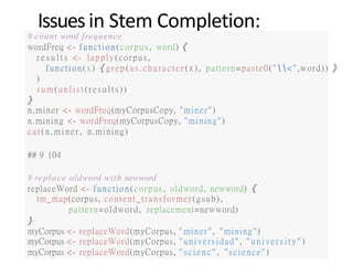
11. Stemming and Stem
Completion 2
myCorpus <- tm_map(myCorpus, stemDocument) # stem words
writeLines(strwrap(myCorpus[[190]]$content, 60))
## r r e f e r card data mine now provid l i nk packag cran packag
## mapreduc hadoop ad
stemCompletion2 <- function(x, dictionary ) { x
<- u n l i s t ( s t r s p l i t ( a s . c h a r a c t e r ( x ) , " " ) ) x
<- x[x != " " ]
x <- stemCompletion(x, dictionary=dictionary)
x <- paste (x, sep="", collapse=" " )
PlainTextDocument(stripWhitespace(x))
}
myCorpus <- lapply(myCorpus, stemCompletion2, dictionary=myCorpusCopy)
myCorpus <- Corpus(VectorSource(myCorpus))
writeLines(strwrap(myCorpus[[190]]$content, 60))
## r reference card data miner now provided l i nk package cran
## package mapreduce hadoop add

12. Issuesin Stem Completion:
“Miner” vs“Mining”
# count word frequence
wordFreq <- function(corpus, word) {
r e s u l t s <- lapply(corpus,
function(x) {grep(as.charac ter ( x) , pattern=paste0("<",word)) }
)
sum (unl is t ( res ul t s))
}
n.miner <- wordFreq(myCorpusCopy, "miner")
n.mining <- wordFreq(myCorpusCopy, "mining")
cat(n.miner, n.mining)
## 9 104
# replace oldword with newword
replaceWord <- function(corpus, oldword, newword) {
tm_map(corpus, content_transformer(gsub),
pattern=oldword, replacement=newword)
}
myCorpus <- replaceWord(myCorpus, "miner", "mining")
myCorpus <- replaceWord(myCorpus, "universidad", "univer s i t y" )
myCorpus <- replaceWord(myCorpus, "scienc" , "science")

13. BUILDING A TERM-DOCUMENT
MATRIX
• A term-document matrix represents the relationship between
terms and documents, where each row stands for a term and
each column for a document, and an entry is the number of
occurrences of the term in the document.
• Alternatively, one can also build a document-term matrix by
swapping row and column. In this section, we build a term-
document matrix from the above processed corpus with
function TermDocumentMatrix(). With its default setting,
terms with less than three characters are discarded. To keep
“r” in the matrix, we set the range of wordLengths in the
example below.

14. Build Term Document Matrix
## data 0 1 0 0 1 0 0 0 0 1
## mining 0 0 0 0 1 0 0 0 0 1
## r 1 1 1 1 0 1 0 1 1 1
tdm <- TermDocumentMatrix(myCorpus,
control = list(wordLengths = c ( 1 , I n f ) ) )
tdm
## <<TermDocumentMatrix (terms: 1073, documents: 448)>>
## Non-/sparse e n t r i e s : 3594/477110
## Sparsity : 99
## Maximal term length: 23
## Weighting : term frequency ( t f )
idx <- which(dimnames(tdm)$Terms i n c ( " r " , "da t a " , "mining"))
as.matrix(tdm[idx, 21:30])
##
## Terms
Docs
21 22 23 24 25 26 27 28 29 30

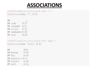
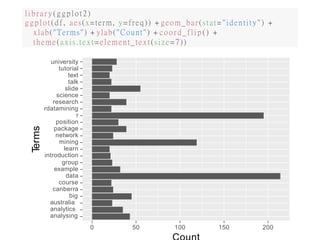
15. Top Frequent Terms :-
We have a look at the popular words and the association betweenwords. Note that
there are 154 tweets in total.
# inspect frequent words
(freq.terms <- findFreqTerms(tdm, lowfreq = 20))
"analytics"
"course"
"a us t r a l i a "
"data"
## [ 1] "analysing"
## [ 5] "canberra"
## [ 9] "group" "introduction" "learn"
## [13] "network"
## [17] "rdatamining"
## [21] "t a l k"
"package"
"research"
"t e xt "
"position"
"science"
" t u t o r i a l "
"big"
"example"
"mining"
" r "
"s l i de "
"university"
term.freq <- rowSums(as.matrix(tdm))
term.freq <- subset (term.freq, term.freq >= 20)
df <- data.frame(term = names(term.freq), freq =term.freq)

16. library(ggplot2)
ggplot (df, aes(x=term, y=freq)) + geom_bar(stat="identity") +
xlab("Terms") + ylab("Count") + coord_flip () +
theme(axis.text=element_text(size=7))
university
tutorial
text
talk
slide
science
research
rdatamining
r
position
package
network
mining
learn
introduction
group
example
data
course
canberra
big
australia
analytics
analysing
0 50 150 200100
Terms

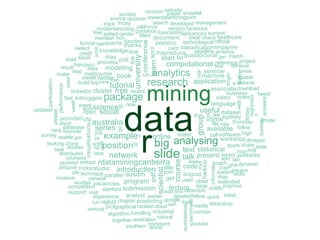
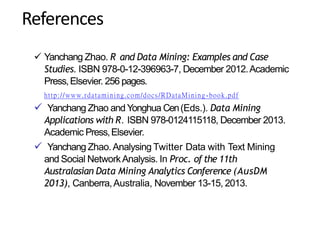
17. WORDCLOUD
• After building a term-document matrix, we can show the importance of
words with a word cloud (also known as a tag cloud), which can be easily
produced with package wordcloud [Fellows, 2012].
• In the code below, we first convert the term-document matrix to a normal
matrix, and then calculate word frequencies.
• After that, we set gray levels based on word frequency and use
wordcloud() to make a plot for it. With wordcloud(), the first two
parameters give a list of words and their frequencies. Words with
frequency below three are not plotted, as specified by min.freq=3. By
setting random.order=F, frequent words are plotted first, which makes
them appear in the center of cloud. We also set the colors to gray levels
based on frequency. A colorful cloud can be generated by setting colors
with rainbow().

18. WordCloud
m<- as.matrix(tdm)
# calculate the frequency of words and sort i t by frequency
word.freq <- sort(rowSums(m), decreasing = T)
# colors
pal <- brewer.pal(9, "BuGn")[-(1:4)]
# plot word cloud
library(wordcloud)
wordcloud(words = names(word.freq), freq = word.freq, min.freq = 3 ,
random.order = F, colors = pa l )

19. data
r
mining
big analysing
network slide
tutorial
course
talk
introduction
series
research application
code
text statistical
available
modeling
program
pdf
scientist
present
time
lecture
august
language
mapreduce
video
workshop
machine
seminar
useful dataset
visualisations
university
conference
learnapril
cfp
australia
join
get
job
postdocthanks
will
analyst
knowledgedue
linkedin cluster free
may
poll
open social
provided
us analytics
database
feb sydney
ieee
hadoop
informal
event scienceth now
stanford submission
outlier call software
create twitter book
find
follow
engin
e
intern
map
recent
thursday
access
acm
area
build topnew can
coursera
experience
file rule
francisco process
add lab
notes
group
tool
webinar
canada
associatedownload
dr
user close extended
fast kdnuggets package
go
high
june
little
nd
distributed iapa
member nov
performance
case
week
senior published
easier detailedfellow quickrisk
short
card classificationsingapore
systemskills
studies vacancies
algorithm handling industrial
amazon tricksrstudio
deadline america
web
today
regressio
n
tuesday
answers
niceaug
australasian
sentiment
competition
credit
dmapps
graph givedynamic
version facebook
retrieval
forest
spatial
titled document page check healthcare
large publicimprove
initial
iselect
link
load excel
looking china
make
step
melbourne
start list postdoctoral jan march
massive
media datacamp
contain
cran mexico
mid
modeinteracting california
neoj keynote
oct positionfit
technological official
participation
please
plotsept extract rdataminingcanberra
pls technique parallel ausdm
computational reference project
result
run sigkdd chapter predicting google topic
format sasapache function
simple
kdd sna detection
source decision wwwrdataminingcom
southern comment
spark share state
sunday
support visit
survey seattle pm
task
together australiannatural
track friday search developed management
tree edited center
guidance forecastingadvanced summit
business tweet
updated
vs examplev online
various profgraphical ranked cloud san
random website
snowfallpaper
world
youtube

20. ASSOCIATIONS
# which words are associated with 'r'?
findAssocs(tdm, " r " , 0.2)
## r
## code 0.27
## example 0.21
## s e r i e s 0.21
## markdown 0.20
## user 0.20
# which words are associated with 'data'?
findAssocs(tdm, "da t a " , 0.2)
##
## mining
## big
data
0.48
0.44
## analytic s 0.31
## science
## pol l
0.29
0.24

21. Network of Terms
library(graph)
l i b r a r y (Rgraphviz)
plot(tdm, term = freq.terms, corThreshold = 0 . 1 , weighting = T)
analysing
analytics
big
canberra coursedata
group
introduction
learnmining
network
example package
australia position
rrdatamining
research
science
slide
talk
text
tutorial
university

22. R packages
 Twitter data extraction: twitteR
 Text cleaning and mining: tm
 Word cloud: wordcloud
 Social network analysis: igraph, sna
 Visualisation: wordcloud, Rgraphviz, ggplot2

23. Twitter Data Extraction – Package twitteR
 userTimeline, homeTimeline, mentions,
retweetsOfMe: retrive various timelines
 getUser, lookupUsers: get information of Twitter user(s)
 getFollowers, getFollowerIDs: retrieve followers (or
their IDs)
 getFriends, getFriendIDs: return alist of Twitter users
(or userIDs) that auser follows
 retweets, retweeters: return retweets or userswho
retweeted atweet
 searchTwitter: issueasearchof Twitter
 getCurRateLimitInfo: retrieve current rate
limit information
 twListToDF: convert into data.frame
https://cran.r-project.org/package=twitteR

24. Text Mining – Package tm
 removeNumbers, removePunctuation, removeWords,
removeSparseTerms, stripWhitespace: remove numbers,
punctuations, wordsor extra whitespaces
 removeSparseTerms: remove sparseterms from a
term-document matrix
 stopwords: various kinds of stopwords
 stemDocument, stemCompletion: stem words
and complete stems
 TermDocumentMatrix, DocumentTermMatrix: build
a term-document matrix or adocument-term matrix
 termFreq: generate aterm frequencyvector
 findFreqTerms, findAssocs: find frequent terms
or associations of terms
 weightBin, weightTf, weightTfIdf, weightSMART,
WeightFunction: various waysto weight aterm-document
matrix

25. Social Network Analysis and Visualization – Package
igraph
degree, betweenness, closeness, t r a n s i t i v i t y :
various centrality scores
 neighborhood: neighborhood of graphvertices
 c l i q u e s , l a r g e s t . c l i q u e s , maximal.cliques,
clique.number: find cliques, ie. complete subgraphs
 c l u s t e r s , n o . c l u s t e r s : maximal connected components of
agraph and the number of them
 fastgreedy.community, spinglass.community:
community detection
 cohesive.blocks: calculate cohesive blocks
 induced.subgraph: create asubgraph of agraph(igraph)
 read.graph, write.graph: read and writ graphs from and to
files of various formats
https://cran.r-project.org/package=igraph

26. References
 Yanchang Zhao. R and Data Mining: Examples and Case
Studies. ISBN 978-0-12-396963-7, December 2012.Academic
Press,Elsevier. 256 pages.
http://www.rdatamining.com/docs/RDataMining -book.pdf
 Yanchang Zhao andYonghua Cen(Eds.). Data Mining
Applications with R. ISBN 978-0124115118, December 2013.
Academic Press,Elsevier.
 Yanchang Zhao.Analysing Twitter Data with Text Mining
and Social NetworkAnalysis. In Proc. of the 11th
Australasian Data Mining Analytics Conference (AusDM
2013), Canberra,Australia, November 13-15, 2013.

27. Online Resources
 Chapter 10 – Text Mining & Chapter 11 – Social Network
Analysis, in book R and Data Mining: Examples and Case
Studies
http://www.rdatamining.com/docs/RDataMining.pdf
 RDataMining Reference Card
http://www.rdatamining.com/docs/RDataMining -reference-card.pdf
 Online documents, books and tutorials
http://www.rdatamining.com/resources/onlinedocs
 Freeonlinecourses
http://www.rdatamining.com/resources/courses
 RDataMining Group on LinkedIn (22,000+ members)
http://group.rdatamining.com
Twitter (2,700+ followers)
@RDataMining