This document discusses algorithm analysis tools. It explains that algorithm analysis is used to determine which of several algorithms to solve a problem is most efficient. Theoretical analysis counts primitive operations to approximate runtime as a function of input size. Common complexity classes like constant, linear, quadratic, and exponential time are defined based on how quickly runtime grows with size. Big-O notation represents the asymptotic upper bound of a function's growth rate to classify algorithms.

1. Data Structures I (CPCS-204)
Week # 2: Algorithm Analysis tools

2. Algorithm Analysis: Motivation
 A problem can be solved in many different ways
 Single problem, many algorithms
 Which of the several algorithms should I
choose?
 We use algorithm analysis to answer this question
o Writing a working program is not good enough
o The program may be inefficient!
o If the program runs on a large data set, then the running time
becomes an issue

3. What is algorithm analysis?
 A methodology to predict the resources that the
algorithm requires
 Computer memory
 Computational time
 We’ll focus on computational time
 It does not mean memory is not important
 Generally, there is a trade-off between the two factors
o Space-time trade-off is a common term

4. How to analyse algorithms?
 Experimental Approach
 Implement algorithms as programs and run them on
computers
 Not a good approach, though!
o Results only for a limited set of test inputs
o Difficult comparisons due to the experiment environments
(need the same computers, same operating systems, etc.)
o Full implementation and execution of an algorithm
 We need an approach which allows us to avoid
experimental study

5. How to analyse algorithms?
 Theoretical Approach
 General methodology for analysing the running time
o Considers all possible inputs
o Evaluates algorithms in a way that is independent from the
hardware and software environments
o Analyses an algorithm without implementing it
 Count only primitive operations used in an algorithm
 Associate each algorithm with a function f(n) that
characterises the running time of the algorithm as a
function of the input size n
o A good approximation of the total number of primitive
operations

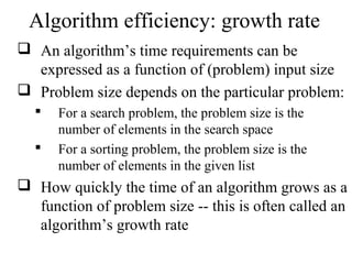
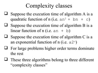
6. Primitive Operations
 Basic computations performed by an algorithm
 Each operation corresponding to a low-level
instruction with a constant execution time
 Largely independent from the programming
language
 Examples
 Evaluating an expression (x + y)
 Assigning a value to a variable (x ←5)
 Comparing two numbers (x < y)
 Indexing into an array (A[i])
 Calling a method (mycalculator.sum())
 Returning from a method (return result)

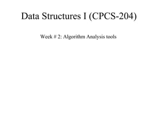
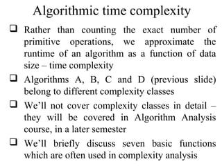
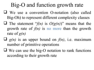
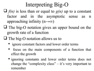
7. Counting Primitive Operations
 Total number of primitive operations executed
 is the running time of an algorithms
 is a function of the input size
 Example
Algorithm ArrayMax(A, n) # operations
currentMax ←A[0] 2: (1 +1)
for i←1;i<n; i←i+1 do 3n-1: (1 + n+2(n- 1))
if A[i]>currentMax then 2(n − 1)
currentMax ←A[i] 2(n − 1)
endif
endfor
return currentMax 1
Total: 7n − 2

8. Algorithm efficiency: growth rate
 An algorithm’s time requirements can be
expressed as a function of (problem) input size
 Problem size depends on the particular problem:
 For a search problem, the problem size is the
number of elements in the search space
 For a sorting problem, the problem size is the
number of elements in the given list
 How quickly the time of an algorithm grows as a
function of problem size -- this is often called an
algorithm’s growth rate

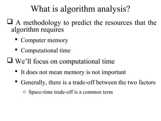
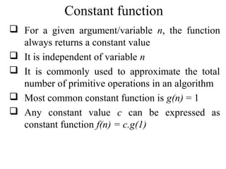
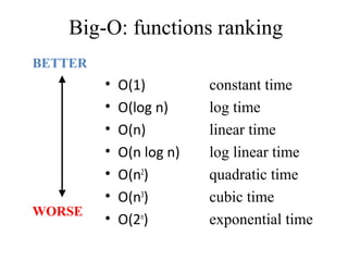
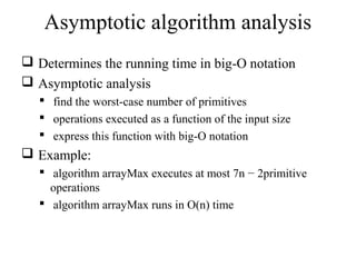
9. Algorithm growth rate
Which algorithm is the most efficient? [The one with
the growth rate Log N.]

10. Algorithmic time complexity
 Rather than counting the exact number of
primitive operations, we approximate the
runtime of an algorithm as a function of data
size – time complexity
 Algorithms A, B, C and D (previous slide)
belong to different complexity classes
 We’ll not cover complexity classes in detail –
they will be covered in Algorithm Analysis
course, in a later semester
 We’ll briefly discuss seven basic functions
which are often used in complexity analysis

11. Seven basic function
1. Constant function f(n) = c
2. Linear function f(n) = n
3. Quadratic function f(n) = n2
4. Cubic function f(n) = n3
5. Log function f(n) = log n
6. Log linear function f(n) = n log n
7. Exponential function f(n) = bn

12. Constant function
 For a given argument/variable n, the function
always returns a constant value
 It is independent of variable n
 It is commonly used to approximate the total
number of primitive operations in an algorithm
 Most common constant function is g(n) = 1
 Any constant value c can be expressed as
constant function f(n) = c.g(1)

13. Linear function
 For a given argument/variable n, the function
always returns n
 This function arises in algorithm analysis any
time we have to do a single basic operation over
each of n elements
 For example, finding min/max value in a list
of values
 Time complexity of linear/sequential search
algorithm is linear

14. Quadratic function
 For a given argument/variable n, the function
always returns square of n
 This function arises in algorithm analysis any
time we use nested loops
 The outer loop performs primitive operations in
linear time; for each iteration, the inner loop also
perform primitive operations in linear time
 For example, sorting an array in
ascending/descending order using Bubble Sort
(more later on)
 Time complexity of most algorithms is quadratic

15. Cubic function
 For a given argument/variable n, the function
always returns n x n x n
 This function is very rarely used in algorithm
analysis
 Rather, a more general class “polynomial” is
often used
o f(n) = a0 + a1n + a2n2 + a3n3 + … + adnd

16. Logarithmic function
 For a given argument/variable n, the function
always returns logarithmic value of n
 Generally, it is written as f(n) = logbn, where b
is base which is often 2
 This function is also very common in
algorithm analysis
 We normally approximate the logbn to a value
x. x is number of times n is divided by b until
the division results in a number less than or
equal to 1
 log327 is 3, since 27/3/3/3 = 1.
 log464 is 3, since 64/4/4/4 = 1
 log212 is 4, since 12/2/2/2/2 = 0.75 ≤ 1

17. Log linear function
 For a given argument/variable n, the function
always returns n log n
 Generally, it is written as f(n) = n logbn, where
b is base which is often 2
 This function is also common in algorithm
analysis
 Growth rate of log linear function is faster as
compared to linear and log functions

18. Exponential function
 For a given argument/variable n, the function
always returns bn, where b is base and n is
power (exponent)
 This function is also common in algorithm
analysis
 Growth rate of exponential function is faster
than all other functions

19. Algorithmic runtime
 Worst-case running time
 measures the maximum number of primitive operations
executed
 The worst case can occur fairly often
o e.g. in searching a database for a particular piece of information
 Best-case running time
 measures the minimum number of primitive operations
executed
o Finding a value in a list, where the value is at the first position
o Sorting a list of values, where values are already in desired order
 Average-case running time
 the efficiency averaged on all possible inputs
 maybe difficult to define what “average” means

20. Complexity classes
 Suppose the execution time of algorithm A is a
quadratic function of n (i.e. an2 + bn + c)
 Suppose the execution time of algorithm B is a
linear function of n (i.e. an + b)
 Suppose the execution time of algorithm C is a
an exponential function of n (i.e. a2n)
 For large problems higher order terms dominate
the rest
 These three algorithms belong to three different
“complexity classes”

21. Big-O and function growth rate
 We use a convention O-notation (also called
Big-Oh) to represent different complexity classes
 The statement “f(n) is O(g(n))” means that the
growth rate of f(n) is no more than the growth
rate of g(n)
 g(n) is an upper bound on f(n), i.e. maximum
number of primitive operations
 We can use the big-O notation to rank functions
according to their growth rate

22. 22
Big-O: functions ranking
• O(1) constant time
• O(log n) log time
• O(n) linear time
• O(n log n) log linear time
• O(n2) quadratic time
• O(n3) cubic time
• O(2n) exponential time
BETTER
WORSE

23. Simplifications
 Keep just one term
 the fastest growing term (dominates the runtime)
 No constant coefficients are kept
 Constant coefficients affected by machines,
languages, etc
 Asymptotic behavior (as n gets large) is determined
entirely by the dominating term
 Example: T(n) = 10 n3 + n2 + 40n + 800
o If n = 1,000, then T(n) = 10,001,040,800
o error is 0.01% if we drop all but the n3 (the
dominating) term

24. Big Oh: some examples
 n3 – 3n = O(n3)
 1 + 4n = O(n)
 7n2 + 10n + 3 = O(n2)
 2n + 10n + 3 = O(2n)

25. Big O: more examples
 f(n) = 7n – 2; 7n - 2 is O(n)
? Find c > 0 and n0 ≥ 1 such that 7n-2 ≤ c•n for n ≥ n0
This is true for c = 7 and n0 = 1
at n = 1, 7-2 ≤ 7; at n = 2, 14 – 2 ≤ 14, and so on
 f(n) = 3 log n + 5; 3 log n + 5 is O(log n)
? Find c > 0 and n0 ≥ 1 such that 3 log n + 5 ≤ c•log n for n ≥ n0
This is true for c = 8 and n0 = 2

26. Interpreting Big-O
 f(n) is less than or equal to g(n) up to a constant
factor and in the asymptotic sense as n
approaching infinity (n→∞)
 The big-O notation gives an upper bound on the
growth rate of a function
 The big-O notation allows us to
 ignore constant factors and lower order terms
 focus on the main components of a function that
effect the growth
 ignoring constants and lower order terms does not
change the “complexity class” – it’s very important to
remember

27. Asymptotic algorithm analysis
 Determines the running time in big-O notation
 Asymptotic analysis
 find the worst-case number of primitives
 operations executed as a function of the input size
 express this function with big-O notation
 Example:
 algorithm arrayMax executes at most 7n − 2primitive
operations
 algorithm arrayMax runs in O(n) time

28. Practice
 Express the following functions in terms of Big-O
notation (a, b and c are constants)
1. f(n) = an2 + bn + c
2. f(n) = 2n + n log n + c
3. f(n) = n log n + b log n + c

29. Outlook
Next week, we’ll discuss arrays and searching algorithms