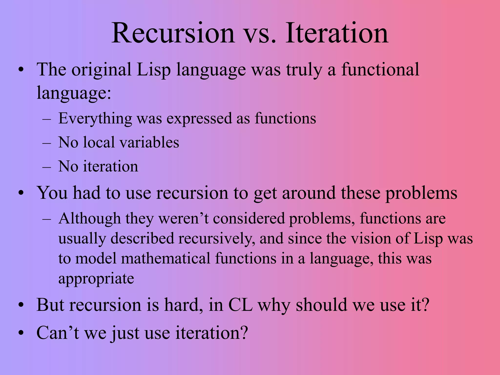
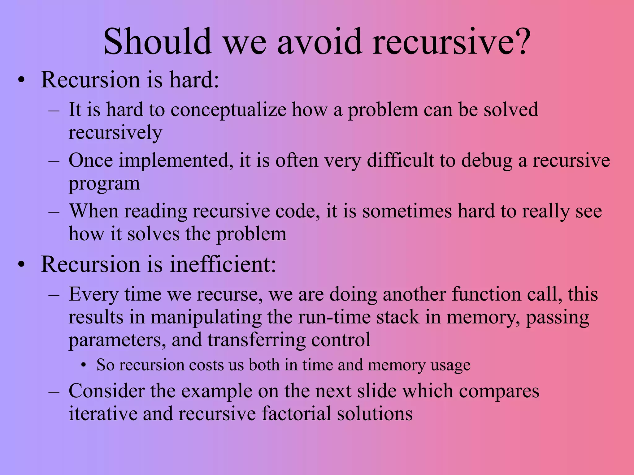
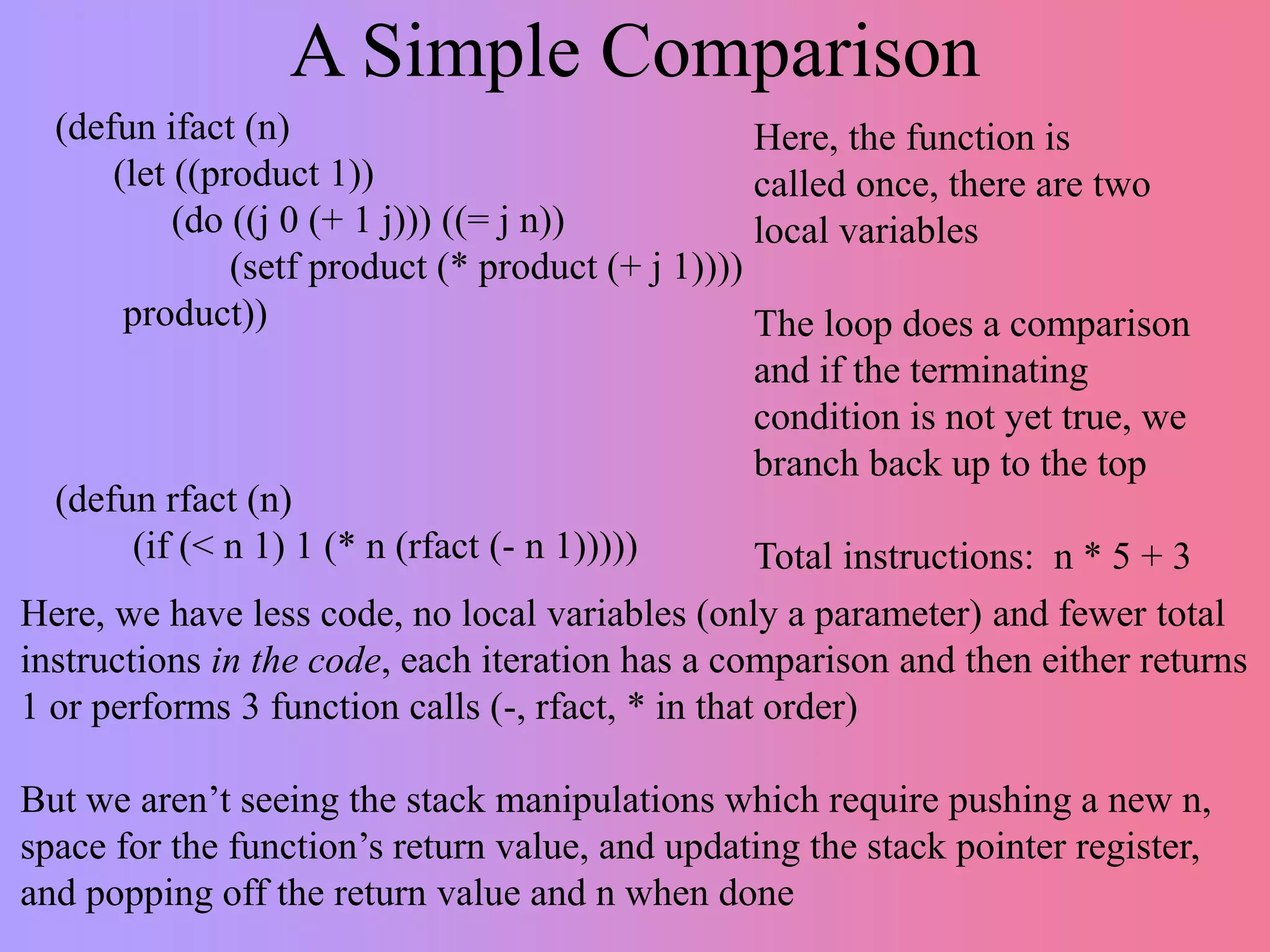
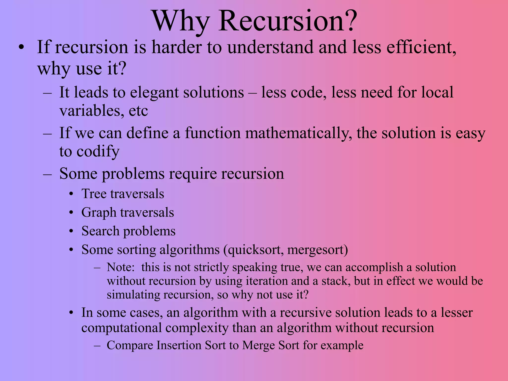
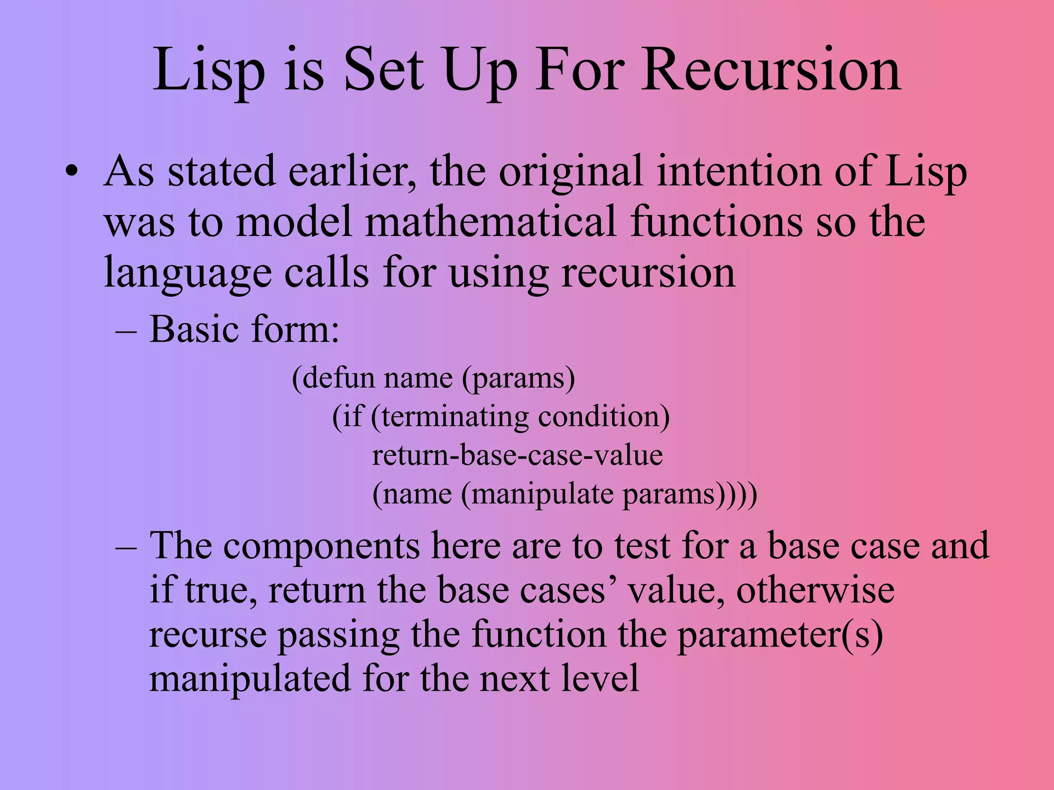
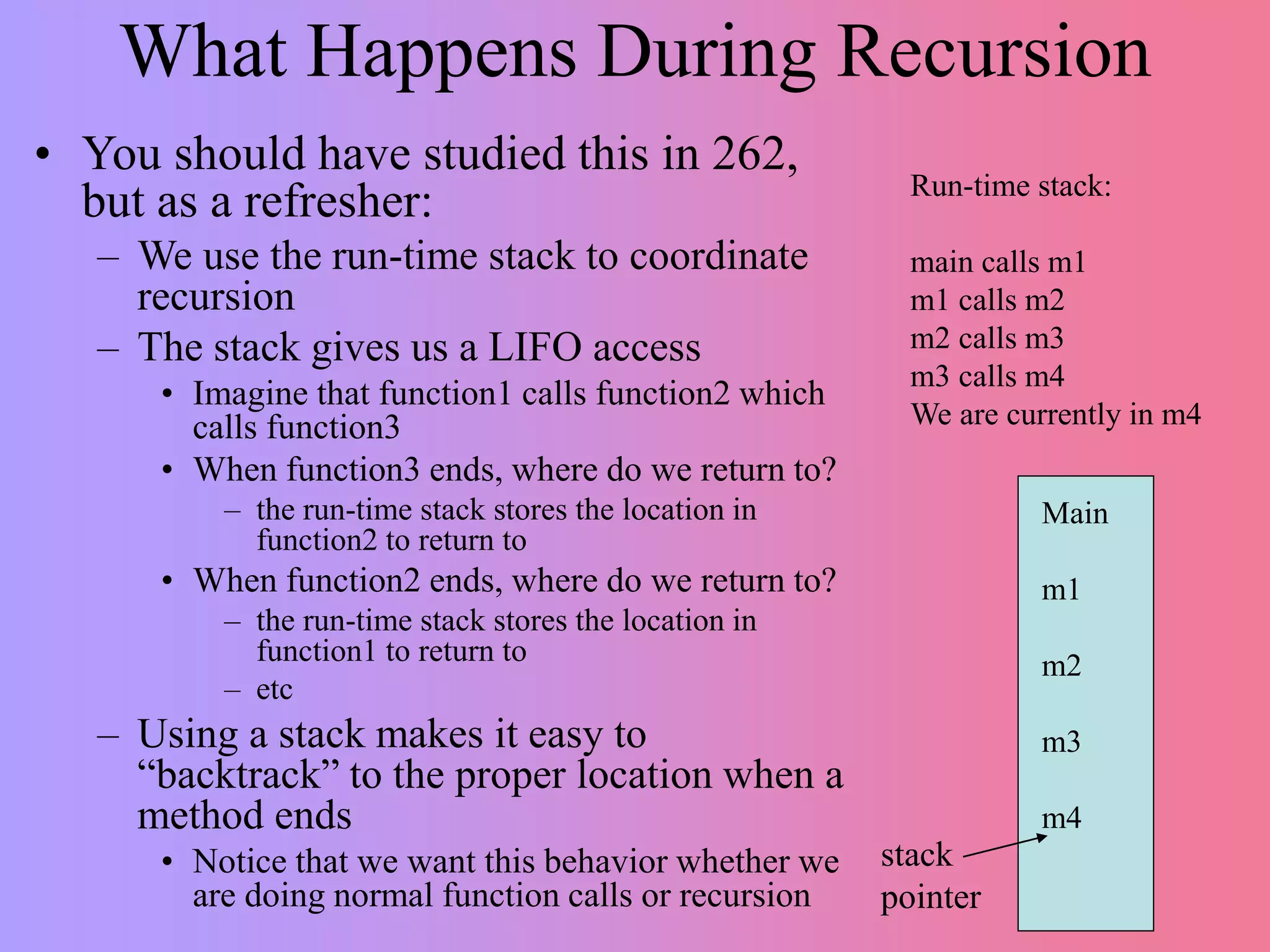
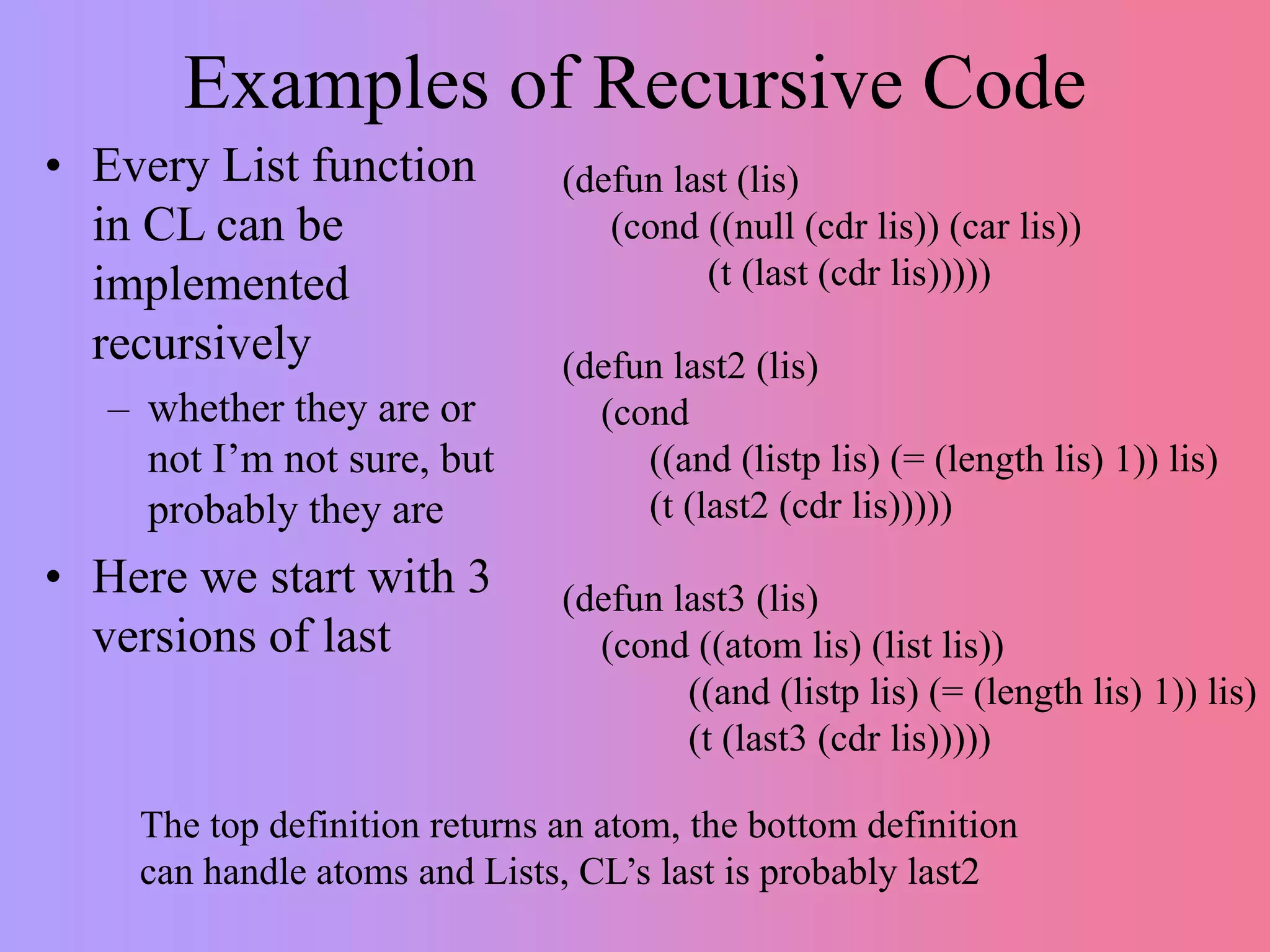
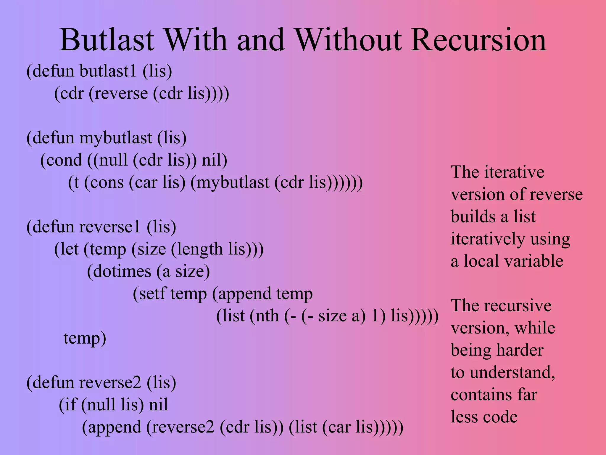
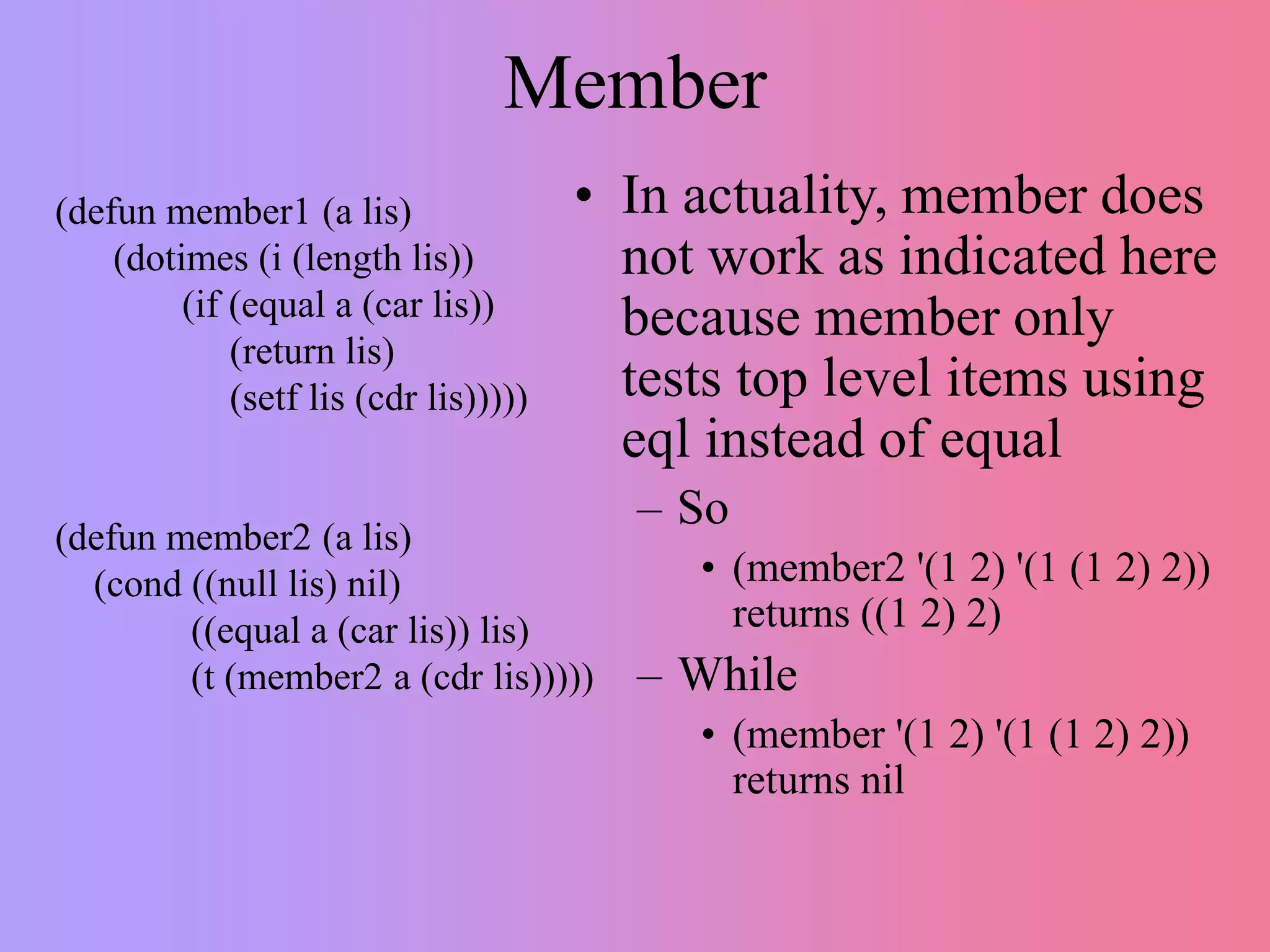
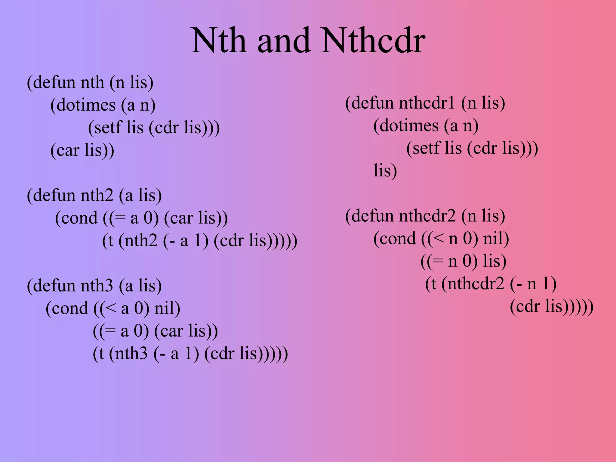
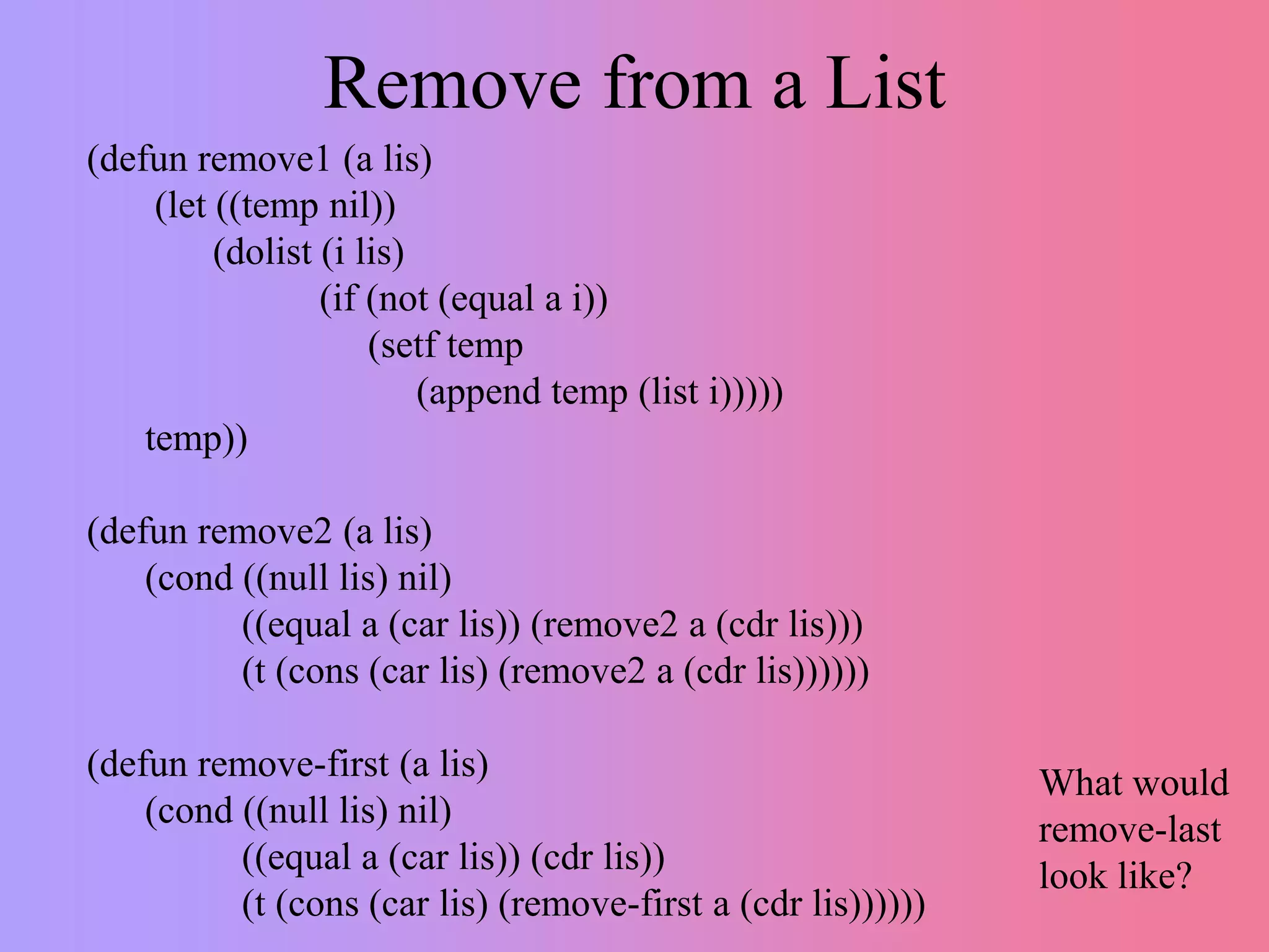
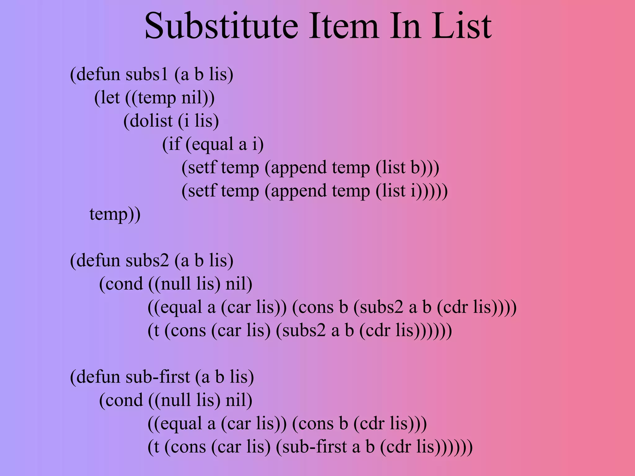
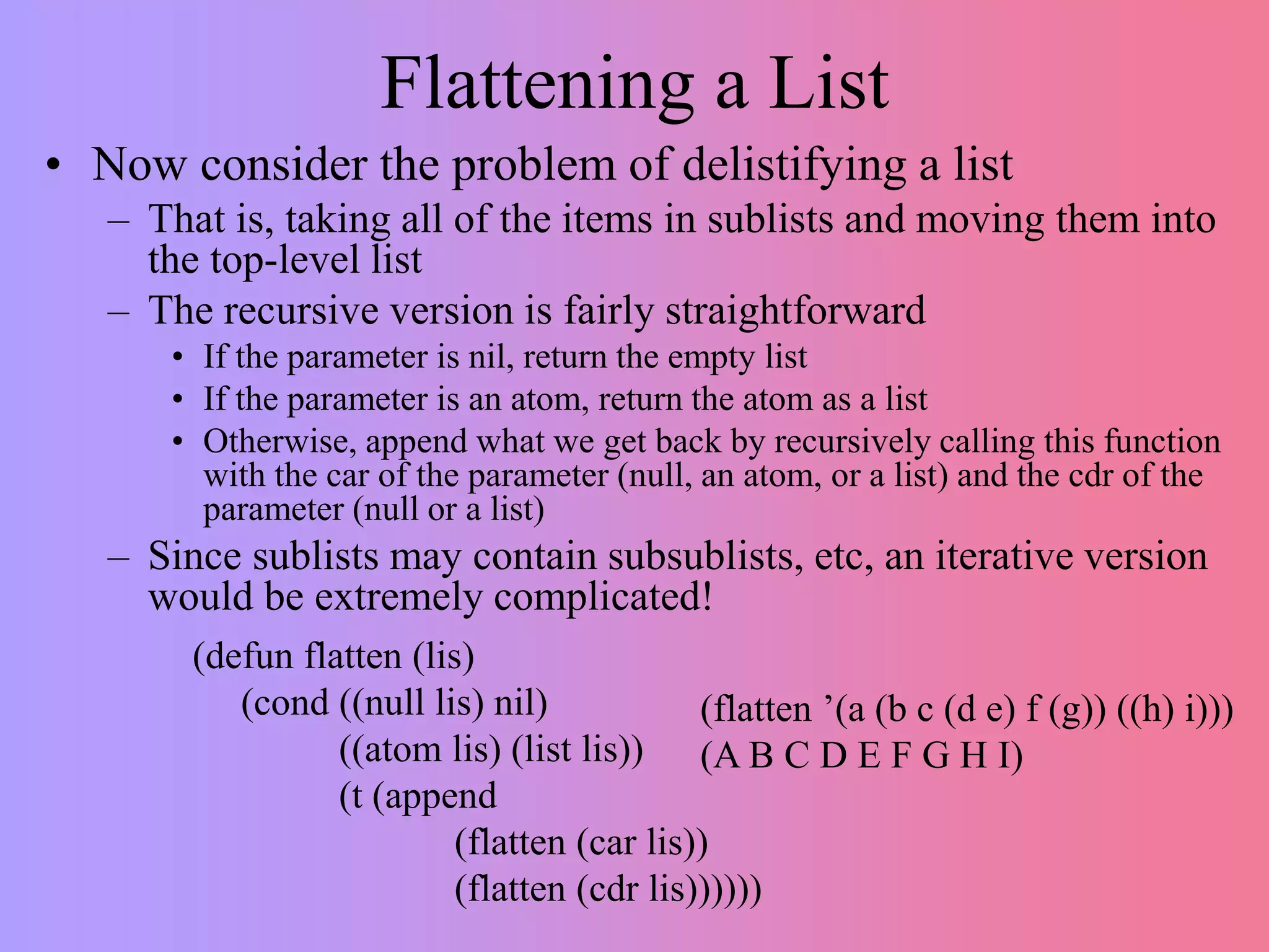
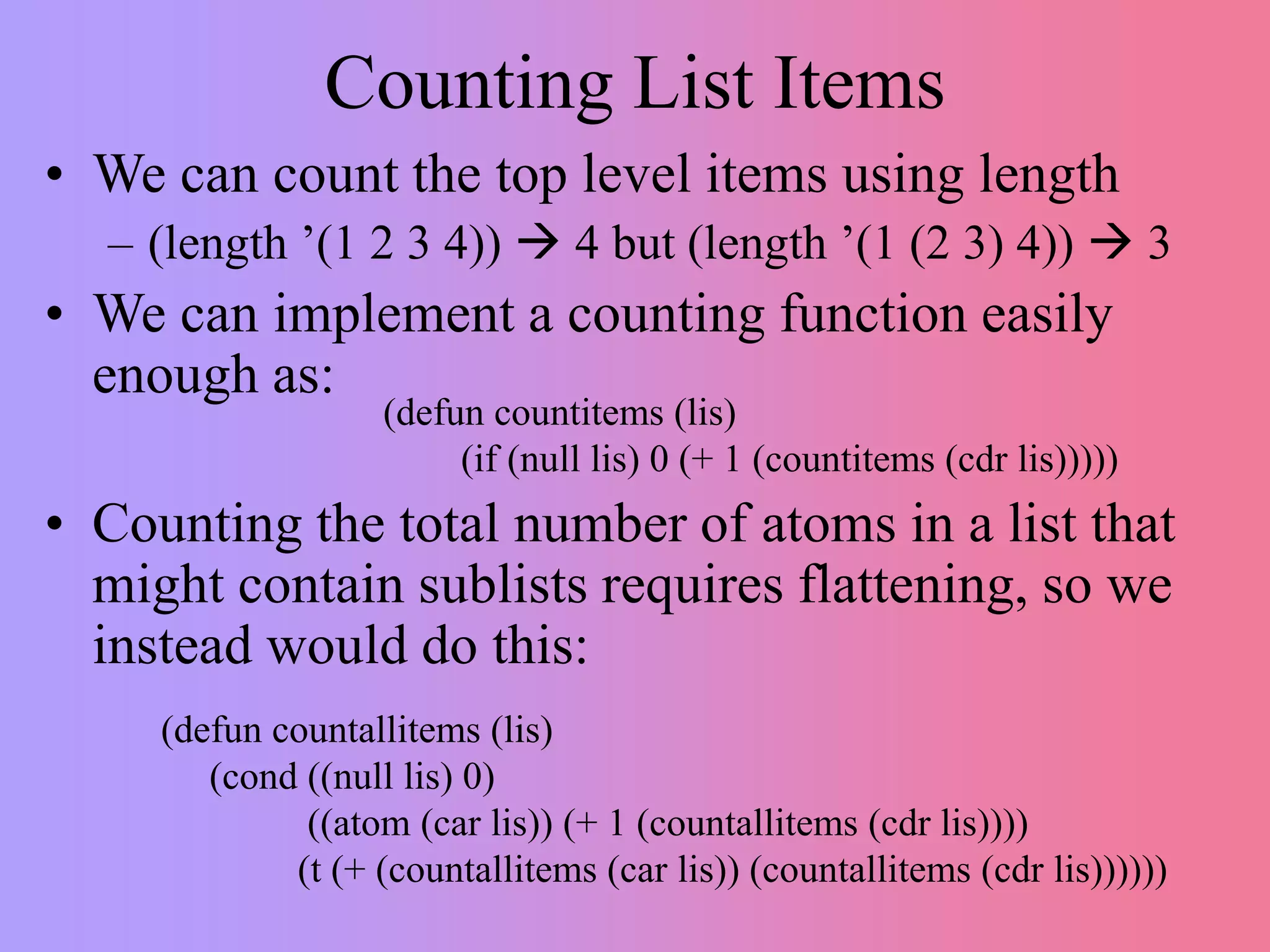
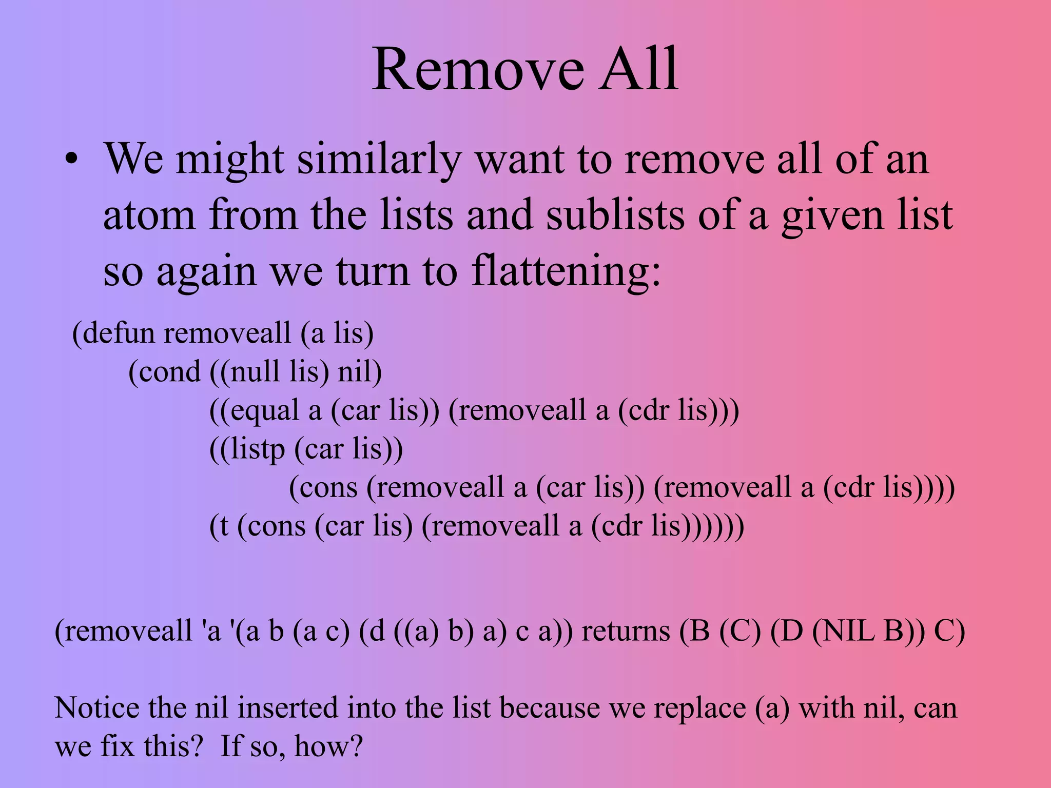
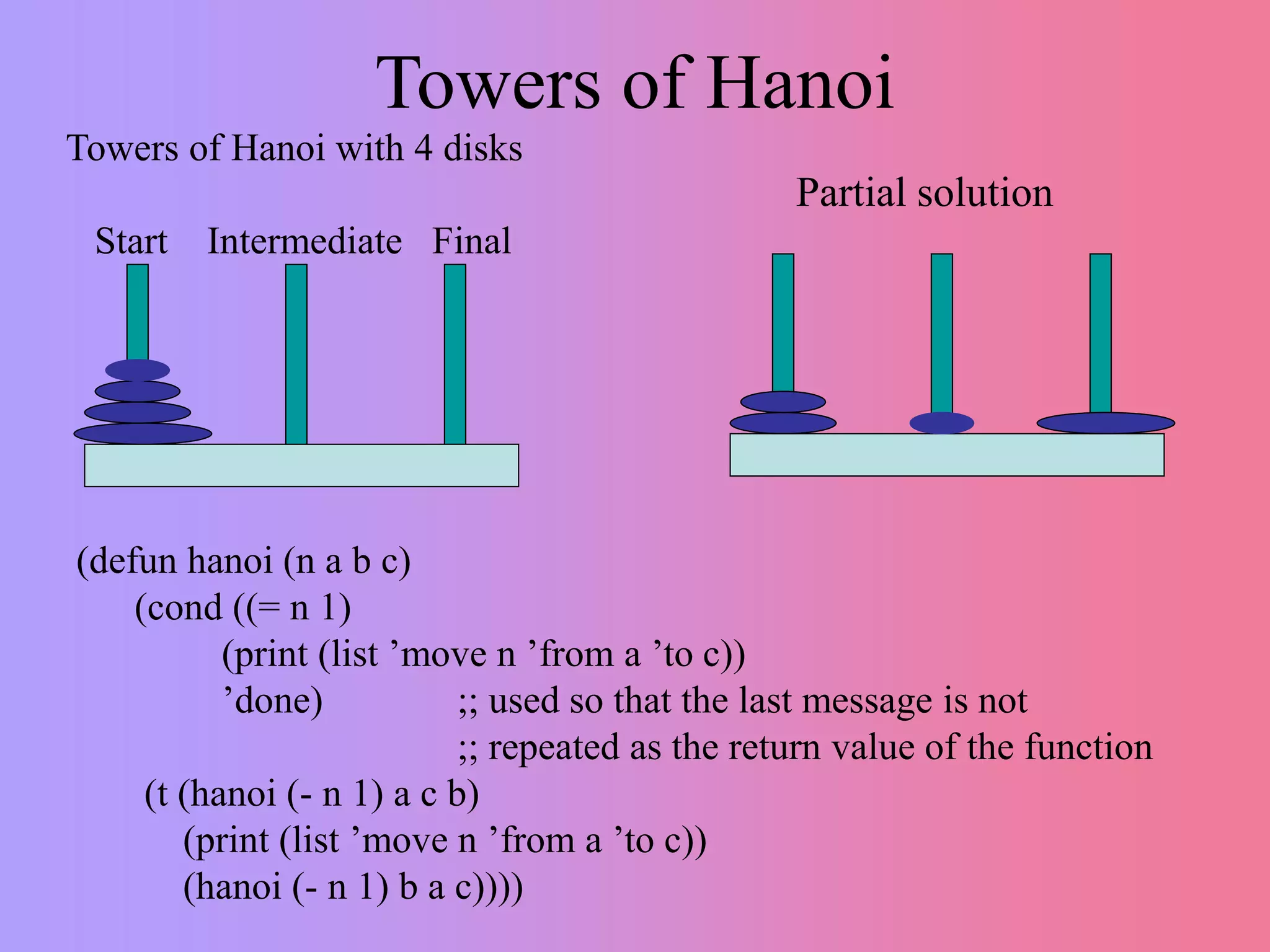
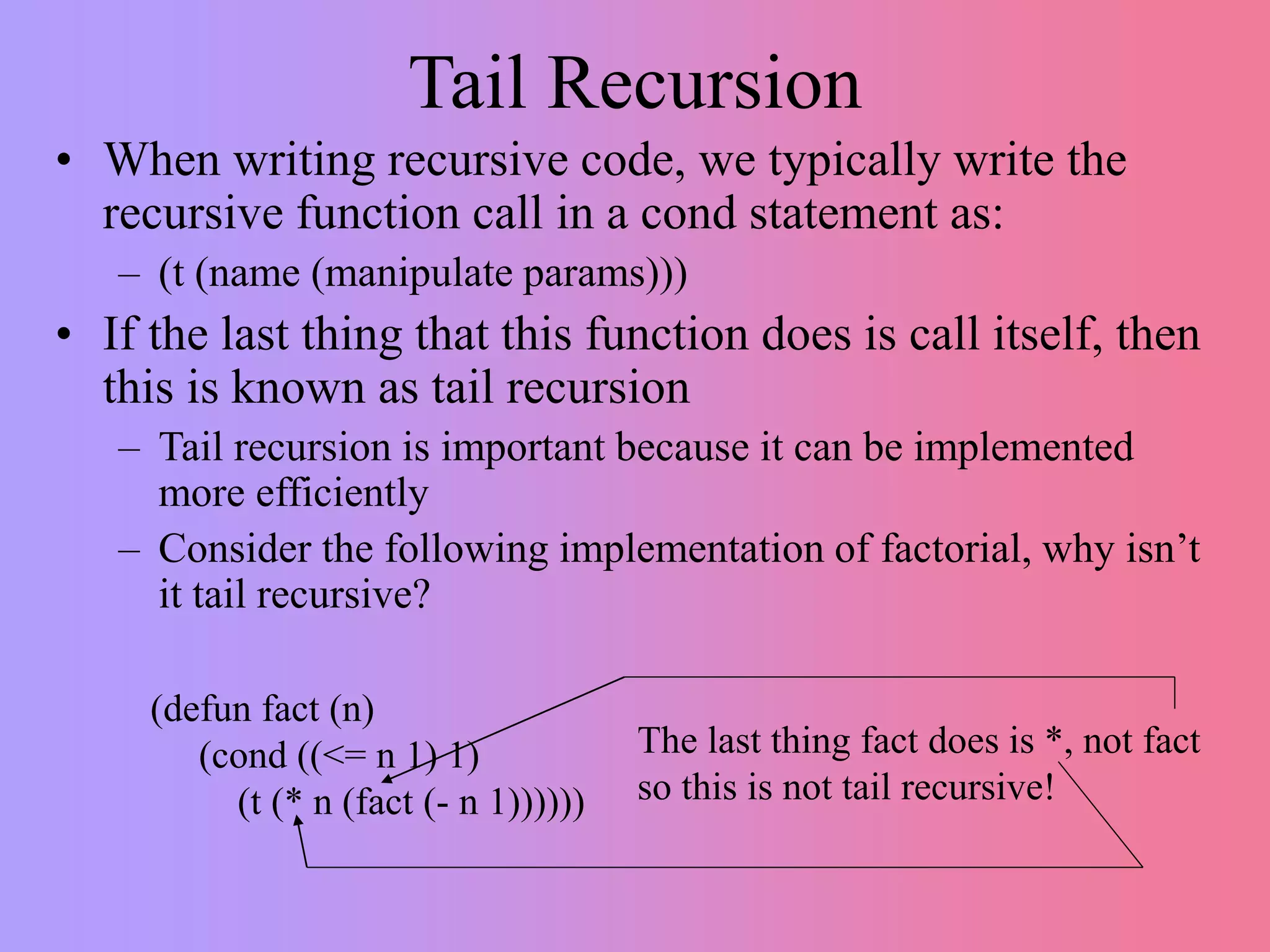
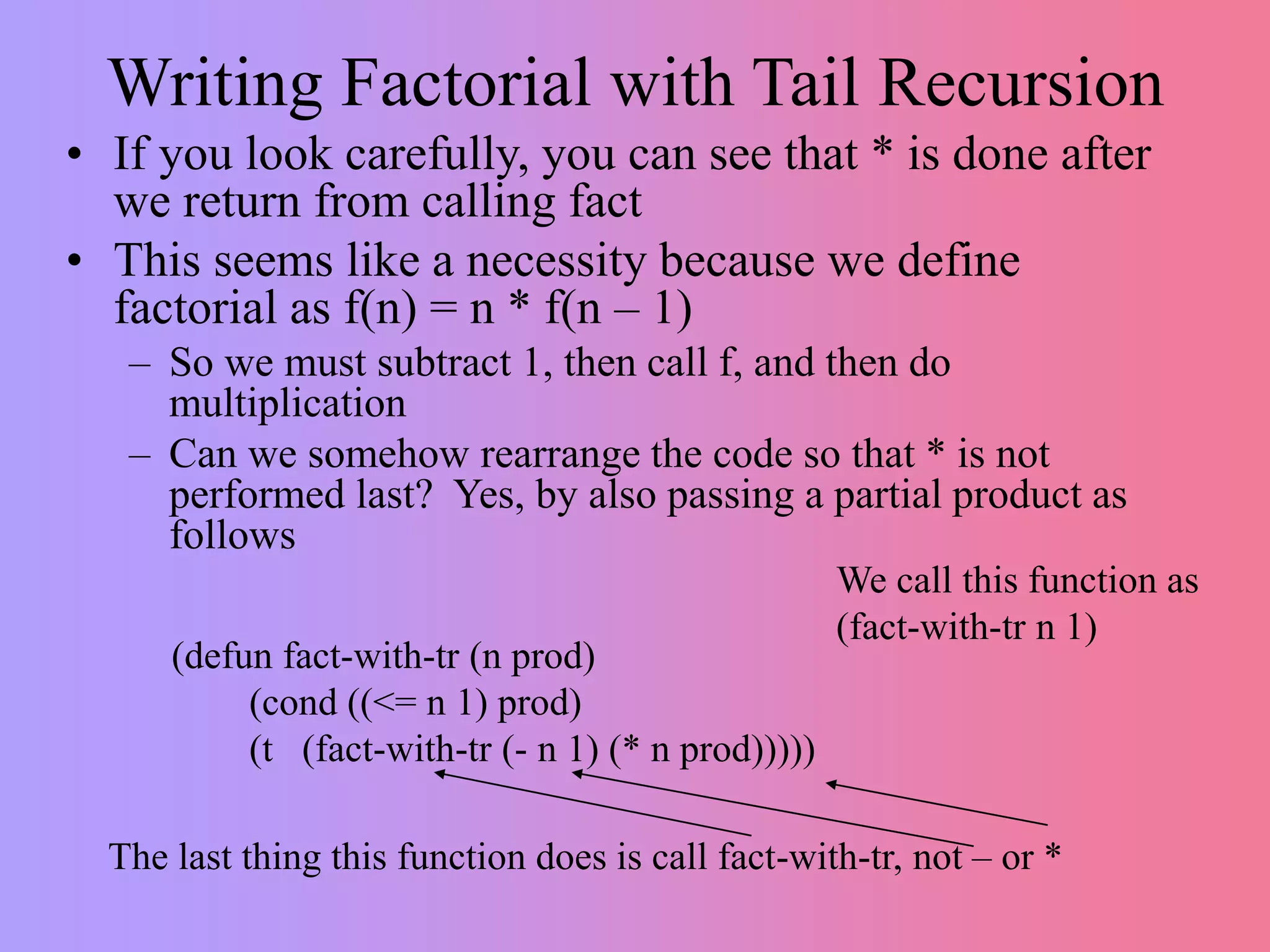
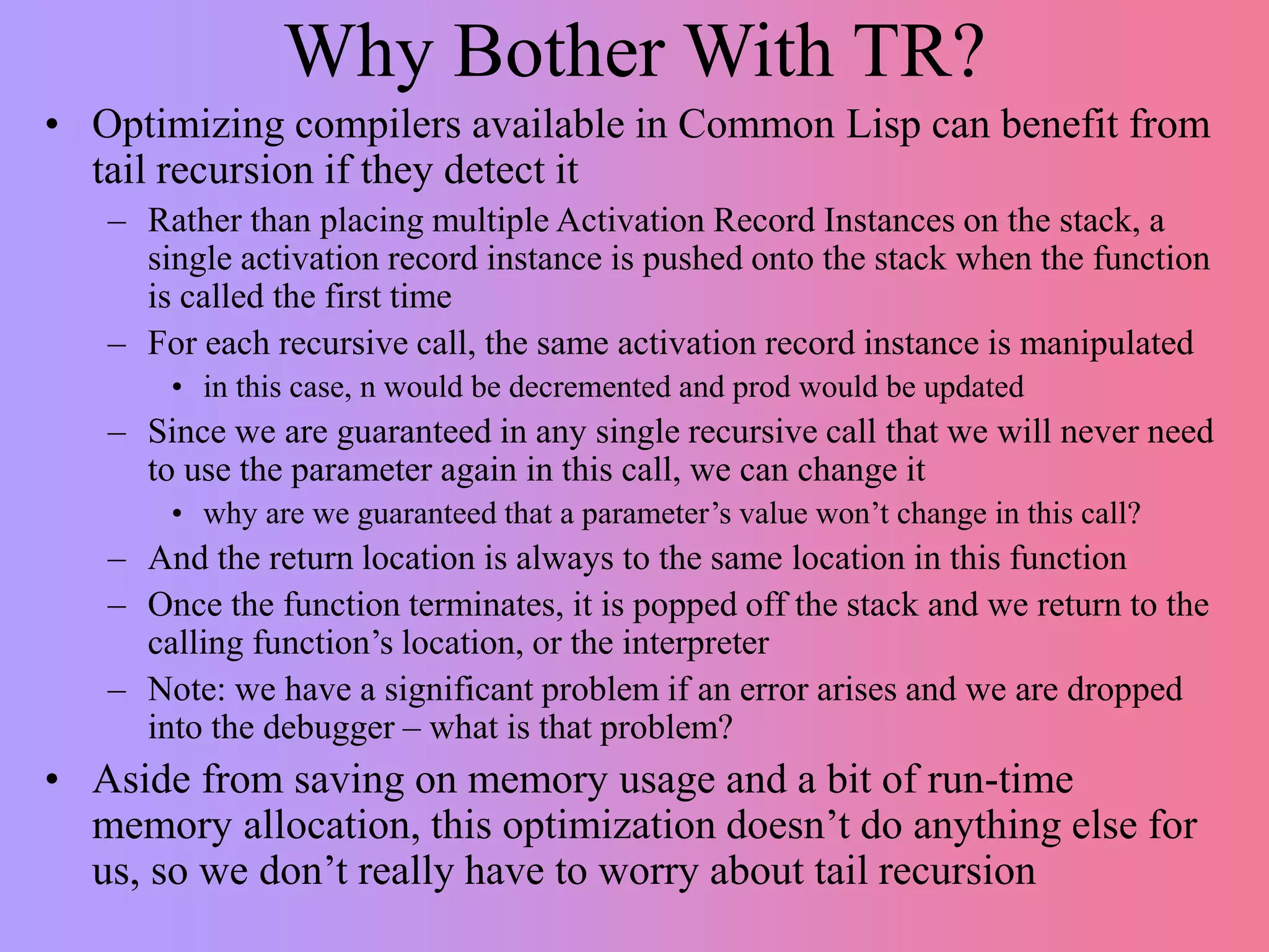
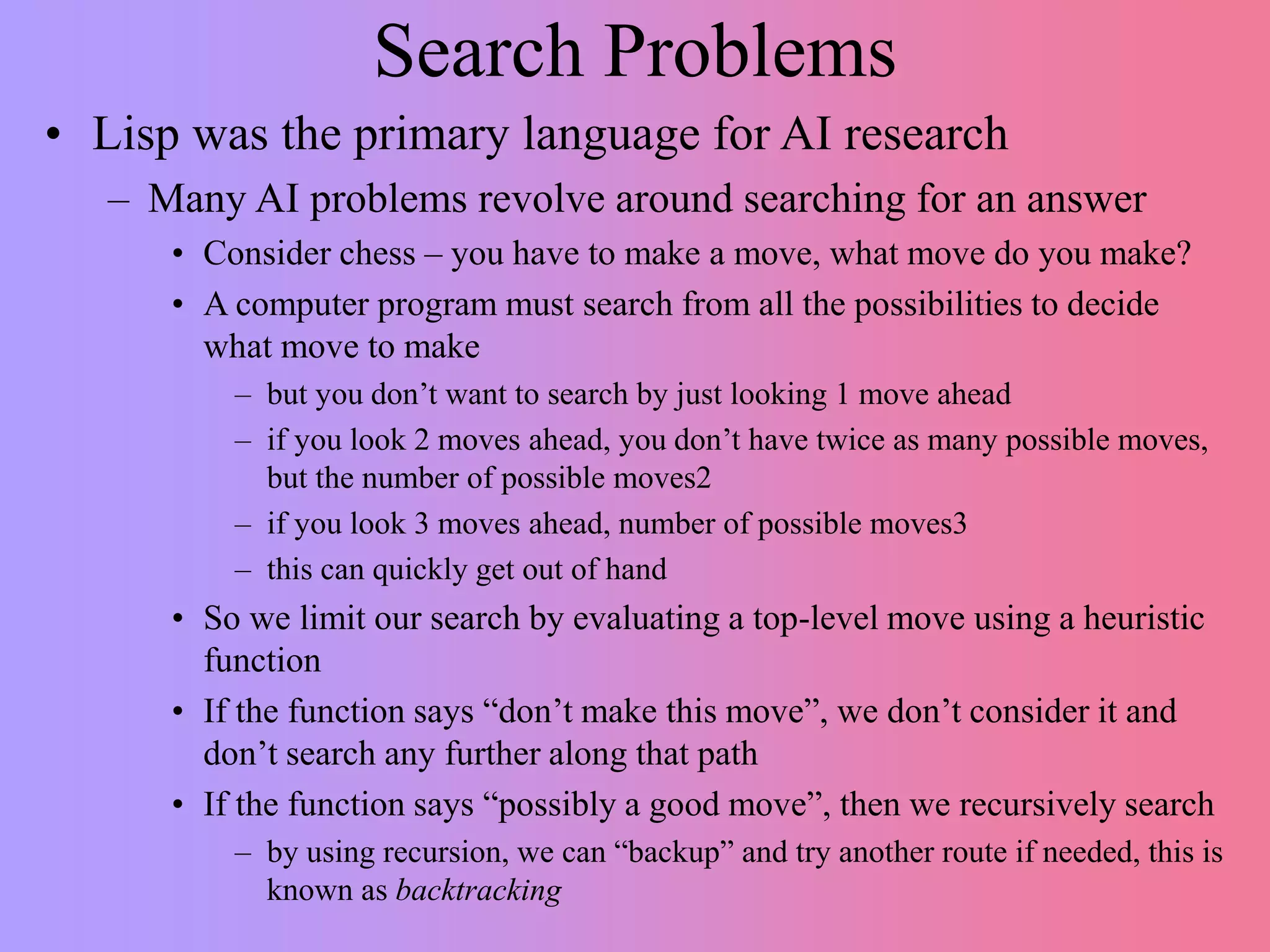
This document discusses recursion versus iteration in Lisp and Common Lisp. It notes that the original Lisp language was purely functional and used recursion to solve problems since it lacked local variables and iteration. While recursion is more elegant and leads to less code in some cases, it is also harder to understand, debug, and less efficient due to function call overhead. However, recursion is necessary for some problems like tree and graph traversals. Common Lisp makes recursion easier through its runtime stack and debugger. Several examples of recursive functions are provided, including ones for lists, trees, searching, and factorials. Tail recursion is discussed as a way to make recursion more efficient.

1. Recursion vs. Iteration
• The original Lisp language was truly a functional
language:
– Everything was expressed as functions
– No local variables
– No iteration
• You had to use recursion to get around these problems
– Although they weren’t considered problems, functions are
usually described recursively, and since the vision of Lisp was
to model mathematical functions in a language, this was
appropriate
• But recursion is hard, in CL why should we use it?
• Can’t we just use iteration?

2. Should we avoid recursive?
• Recursion is hard:
– It is hard to conceptualize how a problem can be solved
recursively
– Once implemented, it is often very difficult to debug a recursive
program
– When reading recursive code, it is sometimes hard to really see
how it solves the problem
• Recursion is inefficient:
– Every time we recurse, we are doing another function call, this
results in manipulating the run-time stack in memory, passing
parameters, and transferring control
• So recursion costs us both in time and memory usage
– Consider the example on the next slide which compares
iterative and recursive factorial solutions

3. A Simple Comparison
(defun ifact (n)
(let ((product 1))
(do ((j 0 (+ 1 j))) ((= j n))
(setf product (* product (+ j 1))))
product))
(defun rfact (n)
(if (< n 1) 1 (* n (rfact (- n 1)))))
Here, the function is
called once, there are two
local variables
The loop does a comparison
and if the terminating
condition is not yet true, we
branch back up to the top
Total instructions: n * 5 + 3
Here, we have less code, no local variables (only a parameter) and fewer total
instructions in the code, each iteration has a comparison and then either returns
1 or performs 3 function calls (-, rfact, * in that order)
But we aren’t seeing the stack manipulations which require pushing a new n,
space for the function’s return value, and updating the stack pointer register,
and popping off the return value and n when done

4. Why Recursion?
• If recursion is harder to understand and less efficient,
why use it?
– It leads to elegant solutions – less code, less need for local
variables, etc
– If we can define a function mathematically, the solution is easy
to codify
– Some problems require recursion
• Tree traversals
• Graph traversals
• Search problems
• Some sorting algorithms (quicksort, mergesort)
– Note: this is not strictly speaking true, we can accomplish a solution
without recursion by using iteration and a stack, but in effect we would be
simulating recursion, so why not use it?
• In some cases, an algorithm with a recursive solution leads to a lesser
computational complexity than an algorithm without recursion
– Compare Insertion Sort to Merge Sort for example

5. Lisp is Set Up For Recursion
• As stated earlier, the original intention of Lisp
was to model mathematical functions so the
language calls for using recursion
– Basic form:
– The components here are to test for a base case and
if true, return the base cases’ value, otherwise
recurse passing the function the parameter(s)
manipulated for the next level
(defun name (params)
(if (terminating condition)
return-base-case-value
(name (manipulate params))))

6. What Happens During Recursion
• You should have studied this in 262,
but as a refresher:
– We use the run-time stack to coordinate
recursion
– The stack gives us a LIFO access
• Imagine that function1 calls function2 which
calls function3
• When function3 ends, where do we return to?
– the run-time stack stores the location in
function2 to return to
• When function2 ends, where do we return to?
– the run-time stack stores the location in
function1 to return to
– etc
– Using a stack makes it easy to
“backtrack” to the proper location when a
method ends
• Notice that we want this behavior whether we
are doing normal function calls or recursion
Run-time stack:
main calls m1
m1 calls m2
m2 calls m3
m3 calls m4
We are currently in m4
Main
m1
m2
m3
m4
stack
pointer

7. More On the Run-time Stack
• For each active function, the run-time stack stores an “activation
record instance”
– This is a description of the function’s execution and stores
• Local variables, Parameters, Return value
• Return pointer (where to return to in the calling function upon function termination)
• Every time a function (or method in Java) is called
– the run-time stack is manipulated by pushing a new activation record instance
onto it
– proper memory space is allocated on the stack for all local variables and
parameters
– the return pointer is set up
– the stack pointer register is adjusted
• Every time a function terminates
– the run-time stack has the top activation record instance popped off of it,
returning the value that the function returns
– the PC (program counter register) is adjusted to the proper location in the calling
function
– the stack pointer register is adjusted

8. An Example
AR for factorial
n = 3
return value: ___
return to: interpreter
(defun fact (n)
(if (<= n 1) 1
(* n (fact (- n 1)))))
The activation record
instance (AR) for
fact stores three things,
n, the return value,
and the pointer of
where to return to in
the next AR when
fact terminates
We start with (fact 3)
AR for factorial
n = 3
return value: ___
return to: interpreter
AR for factorial
n = 3
return value: ___
return to: interpreter
AR for factorial
n = 2
return value: ___
return to: (fact 3) *
AR for factorial
n = 2
return value: ___
return to: (fact 3) *
AR for factorial
n = 1
return value: ___
return to: (fact 2) *

9. Example Continued
AR for factorial
n = 3
return value: ___
return to: interpreter
AR for factorial
n = 3
return value: ___
return to: interpreter
AR for factorial
n = 2
return value:
return to: (fact 3) *
AR for factorial
n = 1
return value: 1
return to: (fact 2) *
AR for factorial
n = 2
return value: 2
return to: (fact 3) *
6 is returned and
printed in the
interpreter
AR for factorial
n = 3
return value: 6
return to: interpreter

10. Lisp Makes Recursion Easy
• Well, strictly speaking, recursion in Lisp is similar to recursion in
any language
• What Lisp can do for us is give us easy access to the debugger
– You can insert a (break) instruction which forces the evaluation step of the
REPL cycle to stop executing, leaving us in the debugger
– Or, if you have a run-time error, you are automatically placed into the
debugger
– From the debugger you can
• inspect the run-time stack to see what values are there
• return to a previous level of recursive call
• provide a value to be returned
– Thus, you can either determine
• why you got an error by inspecting the stack
• see what is going on in the program by inspecting the stack
• return from an error by inserting a partial or complete solution
• CL can also make a recursive program more efficient (to be
explained later)

11. Examples of Recursive Code
• Every List function
in CL can be
implemented
recursively
– whether they are or
not I’m not sure, but
probably they are
• Here we start with 3
versions of last
(defun last (lis)
(cond ((null (cdr lis)) (car lis))
(t (last (cdr lis)))))
(defun last2 (lis)
(cond
((and (listp lis) (= (length lis) 1)) lis)
(t (last2 (cdr lis)))))
(defun last3 (lis)
(cond ((atom lis) (list lis))
((and (listp lis) (= (length lis) 1)) lis)
(t (last3 (cdr lis)))))
The top definition returns an atom, the bottom definition
can handle atoms and Lists, CL’s last is probably last2

12. Butlast With and Without Recursion
(defun butlast1 (lis)
(cdr (reverse (cdr lis))))
(defun mybutlast (lis)
(cond ((null (cdr lis)) nil)
(t (cons (car lis) (mybutlast (cdr lis))))))
(defun reverse1 (lis)
(let (temp (size (length lis)))
(dotimes (a size)
(setf temp (append temp
(list (nth (- (- size a) 1) lis)))))
temp)
(defun reverse2 (lis)
(if (null lis) nil
(append (reverse2 (cdr lis)) (list (car lis)))))
The iterative
version of reverse
builds a list
iteratively using
a local variable
The recursive
version, while
being harder
to understand,
contains far
less code

13. Member
(defun member1 (a lis)
(dotimes (i (length lis))
(if (equal a (car lis))
(return lis)
(setf lis (cdr lis)))))
(defun member2 (a lis)
(cond ((null lis) nil)
((equal a (car lis)) lis)
(t (member2 a (cdr lis)))))
• In actuality, member does
not work as indicated here
because member only
tests top level items using
eql instead of equal
– So
• (member2 '(1 2) '(1 (1 2) 2))
returns ((1 2) 2)
– While
• (member '(1 2) '(1 (1 2) 2))
returns nil

14. Nth and Nthcdr
(defun nth (n lis)
(dotimes (a n)
(setf lis (cdr lis)))
(car lis))
(defun nth2 (a lis)
(cond ((= a 0) (car lis))
(t (nth2 (- a 1) (cdr lis)))))
(defun nth3 (a lis)
(cond ((< a 0) nil)
((= a 0) (car lis))
(t (nth3 (- a 1) (cdr lis)))))
(defun nthcdr1 (n lis)
(dotimes (a n)
(setf lis (cdr lis)))
lis)
(defun nthcdr2 (n lis)
(cond ((< n 0) nil)
((= n 0) lis)
(t (nthcdr2 (- n 1)
(cdr lis)))))

15. Remove from a List
(defun remove1 (a lis)
(let ((temp nil))
(dolist (i lis)
(if (not (equal a i))
(setf temp
(append temp (list i)))))
temp))
(defun remove2 (a lis)
(cond ((null lis) nil)
((equal a (car lis)) (remove2 a (cdr lis)))
(t (cons (car lis) (remove2 a (cdr lis))))))
(defun remove-first (a lis)
(cond ((null lis) nil)
((equal a (car lis)) (cdr lis))
(t (cons (car lis) (remove-first a (cdr lis))))))
What would
remove-last
look like?

16. Substitute Item In List
(defun subs1 (a b lis)
(let ((temp nil))
(dolist (i lis)
(if (equal a i)
(setf temp (append temp (list b)))
(setf temp (append temp (list i)))))
temp))
(defun subs2 (a b lis)
(cond ((null lis) nil)
((equal a (car lis)) (cons b (subs2 a b (cdr lis))))
(t (cons (car lis) (subs2 a b (cdr lis))))))
(defun sub-first (a b lis)
(cond ((null lis) nil)
((equal a (car lis)) (cons b (cdr lis)))
(t (cons (car lis) (sub-first a b (cdr lis))))))

17. Flattening a List
• Now consider the problem of delistifying a list
– That is, taking all of the items in sublists and moving them into
the top-level list
– The recursive version is fairly straightforward
• If the parameter is nil, return the empty list
• If the parameter is an atom, return the atom as a list
• Otherwise, append what we get back by recursively calling this function
with the car of the parameter (null, an atom, or a list) and the cdr of the
parameter (null or a list)
– Since sublists may contain subsublists, etc, an iterative version
would be extremely complicated!
(defun flatten (lis)
(cond ((null lis) nil)
((atom lis) (list lis))
(t (append
(flatten (car lis))
(flatten (cdr lis))))))
(flatten ’(a (b c (d e) f (g)) ((h) i)))
(A B C D E F G H I)

18. Counting List Items
• We can count the top level items using length
– (length ’(1 2 3 4))  4 but (length ’(1 (2 3) 4))  3
• We can implement a counting function easily
enough as:
• Counting the total number of atoms in a list that
might contain sublists requires flattening, so we
instead would do this:
(defun countitems (lis)
(if (null lis) 0 (+ 1 (countitems (cdr lis)))))
(defun countallitems (lis)
(cond ((null lis) 0)
((atom (car lis)) (+ 1 (countallitems (cdr lis))))
(t (+ (countallitems (car lis)) (countallitems (cdr lis))))))

19. Remove All
• We might similarly want to remove all of an
atom from the lists and sublists of a given list
so again we turn to flattening:
(defun removeall (a lis)
(cond ((null lis) nil)
((equal a (car lis)) (removeall a (cdr lis)))
((listp (car lis))
(cons (removeall a (car lis)) (removeall a (cdr lis))))
(t (cons (car lis) (removeall a (cdr lis))))))
(removeall 'a '(a b (a c) (d ((a) b) a) c a)) returns (B (C) (D (NIL B)) C)
Notice the nil inserted into the list because we replace (a) with nil, can
we fix this? If so, how?

20. Towers of Hanoi
(defun hanoi (n a b c)
(cond ((= n 1)
(print (list ’move n ’from a ’to c))
’done) ;; used so that the last message is not
;; repeated as the return value of the function
(t (hanoi (- n 1) a c b)
(print (list ’move n ’from a ’to c))
(hanoi (- n 1) b a c))))
Partial solution
Towers of Hanoi with 4 disks
Start Intermediate Final

21. Tail Recursion
• When writing recursive code, we typically write the
recursive function call in a cond statement as:
– (t (name (manipulate params)))
• If the last thing that this function does is call itself, then
this is known as tail recursion
– Tail recursion is important because it can be implemented
more efficiently
– Consider the following implementation of factorial, why isn’t
it tail recursive?
(defun fact (n)
(cond ((<= n 1) 1)
(t (* n (fact (- n 1))))))
The last thing fact does is *, not fact
so this is not tail recursive!

22. Writing Factorial with Tail Recursion
• If you look carefully, you can see that * is done after
we return from calling fact
• This seems like a necessity because we define
factorial as f(n) = n * f(n – 1)
– So we must subtract 1, then call f, and then do
multiplication
– Can we somehow rearrange the code so that * is not
performed last? Yes, by also passing a partial product as
follows
(defun fact-with-tr (n prod)
(cond ((<= n 1) prod)
(t (fact-with-tr (- n 1) (* n prod)))))
The last thing this function does is call fact-with-tr, not – or *
We call this function as
(fact-with-tr n 1)

23. Why Bother With TR?
• Optimizing compilers available in Common Lisp can benefit from
tail recursion if they detect it
– Rather than placing multiple Activation Record Instances on the stack, a
single activation record instance is pushed onto the stack when the function
is called the first time
– For each recursive call, the same activation record instance is manipulated
• in this case, n would be decremented and prod would be updated
– Since we are guaranteed in any single recursive call that we will never need
to use the parameter again in this call, we can change it
• why are we guaranteed that a parameter’s value won’t change in this call?
– And the return location is always to the same location in this function
– Once the function terminates, it is popped off the stack and we return to the
calling function’s location, or the interpreter
– Note: we have a significant problem if an error arises and we are dropped
into the debugger – what is that problem?
• Aside from saving on memory usage and a bit of run-time
memory allocation, this optimization doesn’t do anything else for
us, so we don’t really have to worry about tail recursion

24. Search Problems
• Lisp was the primary language for AI research
– Many AI problems revolve around searching for an answer
• Consider chess – you have to make a move, what move do you make?
• A computer program must search from all the possibilities to decide
what move to make
– but you don’t want to search by just looking 1 move ahead
– if you look 2 moves ahead, you don’t have twice as many possible moves,
but the number of possible moves2
– if you look 3 moves ahead, number of possible moves3
– this can quickly get out of hand
• So we limit our search by evaluating a top-level move using a heuristic
function
• If the function says “don’t make this move”, we don’t consider it and
don’t search any further along that path
• If the function says “possibly a good move”, then we recursively search
– by using recursion, we can “backup” and try another route if needed, this is
known as backtracking