Downloaded 28 times


![The Algorithm of Bucket-SORT
BUCKET SORT (A)
1. Let B[0..n – 1] be a new array
2. N = A.length
3. For I = 0 to n – 1
4. make B[i] an empty list
5. For I = 1 to n
6. insert A[i] into list B[[nA[i]]]
7. For I = 0 to n – 1
8. sort list B[i] with insertion sort
9. Concatenate the lists B[0], B[1],..B[n-1] together in order.](https://image.slidesharecdn.com/sortingppt-170503171150/85/Sorting-ppt-12-320.jpg)
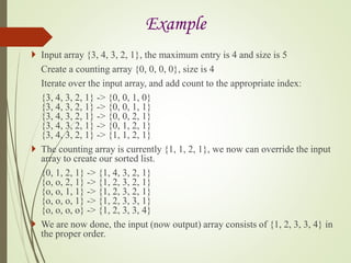
![Example
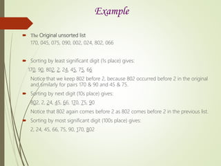
Short Example of a Quick sort Routine (Pivots chosen "randomly")
Input: [13 81 92 65 43 31 57 26 75 0]
Pivot: 65
Partition: [13 0 26 43 31 57] 65 [ 92 75 81]
Pivot: 31 81
Partition: [13 0 26] 31 [43 57] 65 [75] 81 [92]
Pivot: 13
Partition: [0] 13 [26] 31 [43 57] 65 [75] 81 [92]
Combine: [0 13 26] 31 [43 57] 65 [75 81 92]
Combine: [0 13 26 31 43 57] 65 [75 81 92]
Combine: [0 13 26 31 43 57 65 75 81 92]](https://image.slidesharecdn.com/sortingppt-170503171150/85/Sorting-ppt-14-320.jpg)
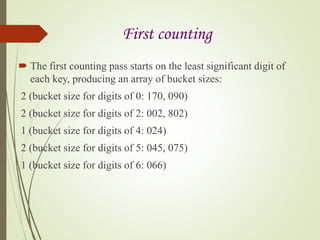
![• Divide Step
If a given array A has zero or one element, simply return; it is
already sorted. Otherwise, split A[p .. r] into two
subarrays A[p .. q] and A[q + 1 .. r], each containing about half
of the elements of A[p .. r]. That is, q is the halfway point
of A[p .. r].](https://image.slidesharecdn.com/sortingppt-170503171150/85/Sorting-ppt-18-320.jpg)
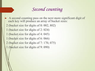
![• Combine Step
Combine the elements back in A[p .. r] by merging the two sorted
subarrays A[p .. q] and A[q + 1 .. r] into a sorted sequence. To
accomplish this step, we will define a procedure MERGE
(A, p, q, r).
• Conquer Step
Conquer by recursively sorting the two subarrays A[p .. q]
and A[q + 1 .. r].](https://image.slidesharecdn.com/sortingppt-170503171150/85/Sorting-ppt-19-320.jpg)
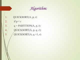
![Algorithm:
MERGE-SORT (A, p, r)
IF p < r // Check for base case
THEN q = FLOOR[(p + r)/2] // Divide step
MERGE (A, p, q) // Conquer step.
MERGE (A, q + 1, r) // Conquer step.
MERGE (A, p, q, r) // Conquer step.](https://image.slidesharecdn.com/sortingppt-170503171150/85/Sorting-ppt-21-320.jpg)
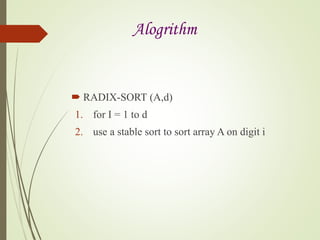
![Algorithm
1. Counting-Sort (A,B,k)
2. For I = 0 to k
3. C[i] = 0
4. For j = 1 to A.length
5. C[A[j]] = C[A[j]] + 1
6. // C[i] now contains the number of elements equal to I
7. For I = 1 to k
8. C[i] = C[i] + C[I – 1]
9. // C[i] now contains the number of elements less than or equal to i.
10. For j = A.length downto 1
11. B[C[A[j]]] = A[j]
12. C[A[j]] = C[A[j]] – 1](https://image.slidesharecdn.com/sortingppt-170503171150/85/Sorting-ppt-24-320.jpg)


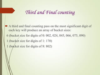
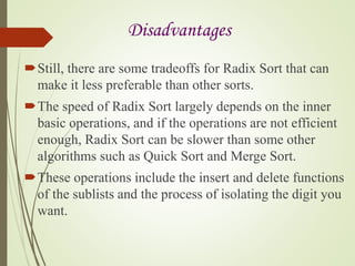
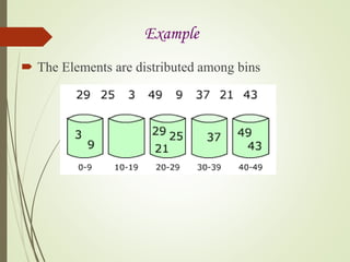
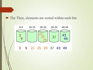
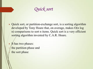
The document describes several sorting algorithms including Radix Sort, Bucket Sort, Quick Sort, Merge Sort, and Counting Sort, detailing their methods and examples. Radix Sort organizes integers by significant digits, while Bucket Sort partitions data into buckets for partial sorting. Quick Sort is efficient with average complexity of O(n log n), and Merge Sort employs a divide and conquer strategy, whereas Counting Sort is focused on sorting small integers based on their keys.


![谷歌留痕技术教程[ 𝙩𝙤𝙥 𝟮𝟯𝟯. 𝙘 𝙤𝙢 ]](https://cdn.slidesharecdn.com/ss_thumbnails/top233-260130173900-2eb784f9-thumbnail.jpg?width=640&height=640&fit=bounds)


