This document discusses choosing appropriate statistical tests based on study design and data type. It covers descriptive studies that measure prevalence and incidence, as well as analytic studies like randomized controlled trials, cohort studies, and case-control studies. For data type, it discusses approaches for continuous and categorical variables, including t-tests, ANOVA, chi-square tests, and regression. It also discusses measures of disease frequency, effect, and impact like risk difference, risk ratio, and odds ratio.

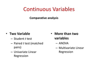
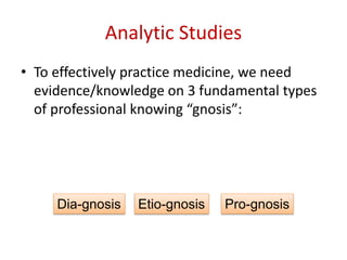
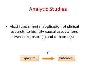
1. Choosing Appropriate Statistical
Test
Amr Albanna, MD, MSc

2. Factors Influencing the Selection of
Statistical Tests
Study Design
Type of Data

3. Study Design

4. 4

5. Descriptive Studies
• Prevalence
– Cross-sectional study
• Incidence
– Cohort study

6. Prevalence Versus Incidence
• Prevalence can be viewed
as describing a pool of
disease in a population.
• Incidence describes the
input flow of new cases
into the pool.
• Deaths and cures reflects
the output flow from the
pool.

7. Prevalence Versus Incidence
Prevalence at time t1 = 2/10 = 20%
Source: Silva 1999
Prevalence at time t2 = 3/8 = 38%
Incidence between t1 and t2: 4/8 = 50%

8. Descriptive Studies
• Determine the size of health problem in the
“study base” population.
• Promote public health policies.

9. Analytic Studies
• Randomized-controlled trials.
• Cohort studies
• Case-control studies
• Diagnostic studies

10. Analytic Studies
• To effectively practice medicine, we need
evidence/knowledge on 3 fundamental types
of professional knowing “gnosis”:
Dia-gnosis Etio-gnosis Pro-gnosis

11. • Most fundamental application of clinical
research: to identify causal associations
between exposure(s) and outcome(s)
Exposure Outcome
?
Analytic Studies

12. Causal Vs. Non-causal Association
A B
Accidental
No Association

13. Causal Vs. Non-causal Association
A B
A cause B

14. Causal Vs. Non-causal Association
A B
B cause A

15. Direction of causality: does overeating cause obesity?
Taubes G
New Scientist
2008

16. Causal Vs. Non-causal Association
A B
A is not causally associated with B
C e.g. Smoking
e.g. Lung cancere.g. Coffee

17. A Research Scenario
• Study question: Does eating affect student
intellectual ability.
• 100 students underwent an exam after eating
lunch.
• 50% failed the exam.
• You conclude that eating worsen students
intellectual ability.

18. Compared to what?
• In an old movie, comedian
Groucho Marx is asked:
“Groucho, how’s your wife?”
• Groucho quips: “Compared
to what?”
http://en.wikipedia.org

19. Outcome
Outcome
Counterfactual, unexposed cohort
Exposed cohort
Ideal counterfactual comparison to determine
causal effects
Maldonado & Greenland, Int J Epi 2002;31:422-29
“Initial conditions” are identical in
the exposed and unexposed groups
– because they are the same
population!

20. Outcome
Outcome
Counterfactual, unexposed cohort
Exposed cohort
Substitute, unexposed cohort
Outcome
What happens in reality?
counterfactual state
is not observed
(latent)
A substitute will usually be a population other than the target population
during the etiologic time period - INITIAL CONDITIONS MAY BE
DIFFERENT

21. Risk
Rate
Risk
Difference
Risk Ratio
Rate Ratio
Odds Ratio

22. Measures
of disease
freq
Measures
of effect
Measures
of potential
impact

23. Attributable Risk

24. Population Attributable Risk

25. How PAR is dependent on prevalence of
exposure
Szklo & Nieto. Epidemiology: Beyond the basics. 2nd Edition, 2007

26. Randomization helps to make the groups “comparable” (i.e. similar
initial conditions)
Eligible patients
Treatment
Randomization
Placebo
Outcomes
Outcomes
Randomized-controlled trials
Incidence
Incidence
Difference: “RR” or “RD”

27. Observational Studies
E
E
E
E
E
E
E
E
EE
E
E
N
E
E
N
N
N
N
N
N
N
N
N
N
N
N
N
N N
N
N
N
N
N
N
N
N
E
E
E
E
E
E
E
E
E
N
NN
N
N
N
N
N

28. Cohort
E
E
E
E
E
E
E
E
E
E
E
E
N
E
E
N
N
N
N N NN
N
N
N
N
NN
N
N
N
N
N
N
N
N
N
N
E
E
E
E
E
E
E
E
E
N
N
N
NN
N
N
N
N
Un-Exposed
Exposed

29. Study population
ExposedUnexposed
Disease
No
Disease
Disease
No
Disease
Incidence of
disease in exposed
Incidence of disease
in unexposed
Cohort
“Risk Ratio”
“Risk Difference”

30. Case-Control
E EE
E
EE
E
E
E
EE
E
N
E
E
N
N
N
N N
N N N
N
N
NN N N N
N
N
N
N N
N
N NE
E E
EE
E E E
E
N
N
N
N
N
N
N
N N
Cases
Controls

31. Study population
DiseaseNo disease
Exposed
Un-
exposed
Exposed
Un-
exposed
Odds of being
exposed
Odds of being
exposed
Case-control
“Odds Ratio”
approximate “Risk Ratio”

32. Observational Studies: Problem
Association between birth order and Down syndrome
Source: Rothman 2002Data from Stark and Mantel (1966)

33. Source: Rothman 2002
Association between maternal age and Down syndrome
Data from Stark and Mantel (1966)

34. Source: Rothman 2002
Association between maternal age and Down syndrome, stratified by
birth order
Data from Stark and Mantel (1966)

35. Criteria to define confounder
• A factor is a confounder if 3 criteria are met:
– a) a confounder must be causally or noncausally associated
with the exposure in the source population;
– b) a confounder must be a causal risk factor (or a surrogate
measure of a cause) for the disease;
– c) a confounder must not be an intermediate cause (in other
words, a confounder must not be an intermediate step in the
causal pathway between the exposure and the disease)

36. Exposure Disease (outcome)
Confounder
Confounding Schematic
E D
C
Szklo M, Nieto JF. Epidemiology: Beyond the basics. Aspen Publishers, Inc., 2000.
Gordis L. Epidemiology. Philadelphia: WB Saunders, 4th Edition.

37. Exposure Confounder
Intermediate cause
E DC
Disease

38. Birth Order Down Syndrome
Confounding factor:
Maternal Age
Confounding Schematic
E D
C

39. HRT use Heart disease
Confounding factor:
SES
Are confounding criteria met?
Association between HRT and heart disease

40. Control of confounding: Outline
• Control at the design stage
– Randomization
– Restriction
– Matching
• Control at the analysis stage
– Conventional approaches
• Stratified analyses
• Multivariate analyses
– Newer approaches
• Propensity scores

41. Observational Study on Vit E and Coronary Heart
Disease
Fitzmaurice, 2004
Crude OR = (50)(384)/(501)(65) = 0.59
Are there potential confounders that can explain this crude OR?

42. Vitamin E CHD
Confounding factor:
Smoking
Stratify on the
confounding
variable
Could reduced smoking among Vit E users partly
explain the observed protective effect?

43. Stratified Analyses (by smoking status)
Fitzmaurice, 2004
OR (smokers) = (11)(200)/(40)(49) = 1.12
OR (non-smokers) = (39)(184)/(461)(16) = 0.97
Stratum 1
Stratum 2

44. Multivariate Analysis

45. •Diagnostic 2 X 2 table*:
Disease + Disease -
Test + True
Positive
False
Positive
Test - False
Negative
True
Negative
*When test results are not dichotomous, then can use ROC curves [see later]
Diagnostic Studies

46. Disease
present
Disease
absent
Test
positive
True
positives
False
positives
Test
negative
False
negative
True
negatives
Sensitivity
[true positive rate]
The proportion of patients with disease who test
positive = P(T+|D+) = TP / (TP+FN)

47. Disease
present
Disease
absent
Test
positive
True
positives
False
positives
Test
negative
False
negative
True
negatives
Specificity
[true negative rate]
The proportion of patients without disease who test
negative: P(T-|D-) = TN / (TN + FP).

48. Disease
present
Disease
absent
Test
positive
True
positives
False
positives
Test
negative
False
negative
True
negatives
Predictive value of a positive test
Proportion of patients with positive tests who have
disease = P(D+|T+) = TP / (TP+FP)

49. Disease
present
Disease
absent
Test
positive
True
positives
False
positives
Test
negative
False
negative
True
negatives
Predictive value of a negative test
Proportion of patients with negative tests who do not have
disease = P(D-|T-) = TN / (TN+FN)

50. Disease
present
Disease
absent
Test
positive
True
positives
False
positives
Test
negative
False
negative
True
negatives
Likelihood Ratio of a Positive
Test
LR+ = TPR / FPR )|Pr(
)|Pr(



DT
DT
LR
How more often a
positive test result
occurs in persons
with compared to
those without the
target condition

51. Disease
present
Disease
absent
Test
positive
True
positives
False
positives
Test
negative
False
negative
True
negatives
Likelihood Ratio of a Negative
Test
LR- = FNR / TNR )|Pr(
)|Pr(



DT
DT
LR
How less likely a
negative test result
is in persons with
the target condition
compared to those
without the target
condition

52. Continuous results:
Receiver operating characteristic (ROC)curve
Blood sugar level
(2-hour after
food) in
mg/100 ml
Sensitivity
(%)
Specificity
(100%)
70
80
90
100
110
120
130
140
150
160
170
180
190
200
98.6
97.1
94.3
88.6
85.7
71.4
64.3
57.1
50.0
47.1
42.9
38.6
34.3
27.1
8.8
25.5
47.6
69.8
84.1
92.5
96.9
99.4
99.6
99.8
100
100
100
100
Area under the curve (AUC) can range from 0.5 (random
chance, or no predictive ability; refers to the 45 degree line
in the ROC plot) to 1 (perfect discrimination/accuracy).
The closer the curve follows the left-hand border and then the
top-border of the ROC space, the more accurate the test. The
closer the curve comes to the 45-degree diagonal of the ROC
space, the less accurate the test.

53. Systematic Review
Bates et al. Arch Intern Med 2007
Meta-analysis

54. Ried K. Aus Fam Phys 2006

55. Type of Data

56. Continuous Variables
• Mean and 95% CI • Median and IQR
Descriptive analysis

57. Continuous Variables
• Two Variable
– Student t test
– Paired t test (matched
pairs)
– Univariate Linear
Regression
• More than two
variables
– ANOVA
– Multivariate Linear
Regression
Comparative analysis

58. Categorical Variables
• Descriptive analysis
– Proportion and 95% CI
• Comparative analysis
– Chi Square test
– Fisher's exact test
– Logistic Regression

59. Incidence Risk Vs. Incidence Rate
Hypothetical cohort of 12 initially disease-free subjects followed
over a 5-year period from 1990 to 1995.
Incidence risk = 5/12 = 42/100 persons
Incidence rate = 5/25 = 20/100 person-year
Kleinbaum et al. ActivEpi

64. Incidence Rate

65. Example
Hypothetical cohort of 12 initially disease-free subjects followed
over a 5-year period from 1990 to 1995.
Kleinbaum et al. ActivEpi
Incidence risk = 5/12 = 0.42 (42 per 100 persons)
Incidence rate = 5/25 = 0.2 per person year

66. Statistical Significance:
P-Value “or” 95% Confidence Interval

67. Hypothesis Testing (P-value)
• Null hypothesis  No difference.
• P-value < 0.05  Reject the null hypothesis
(there is difference).

68. Problems with P-values
• Does not measure the magnitude of the
difference.
• Depends on the sample size.
– Very small difference can become significant by
increasing the sample size.
• Multiple testing will increase the chance of
having positive (significant difference) result
due to random error.

69. Biggest problem!
• We know that the null hypothesis (difference
= zero) is not true.
• We just need enough power (sample size) to
reject the null hypothesis (and make our study
“POSITIVE”).
• Example: 5-years mortality
Group 1 Group 2
0.0021633098649999 0.0021633098649999

70. Confidence Interval
No difference
(equivalent)
Inconclusive
Better
No difference
May be better, not
worse
BetterWorse