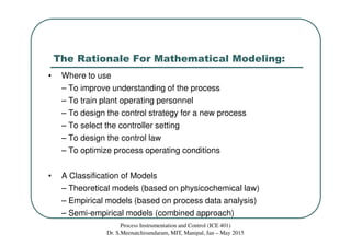
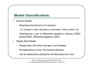
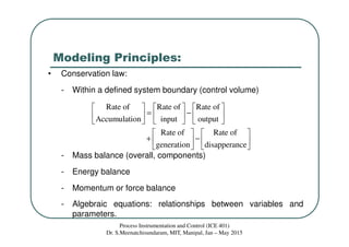
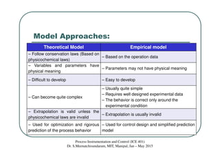
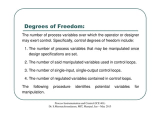
This document discusses mathematical modeling of processes. It describes the rationale for modeling, including improving process understanding, training personnel, and designing control strategies. Models can be theoretical, empirical, or semi-empirical. Dynamic models describe time behavior using differential equations, while steady state models have no time dependency. Modeling principles include conservation laws of mass, energy, and momentum. Theoretical models follow physicochemical laws, while empirical models are based on process data. Degrees of freedom analysis determines the number of variables that can be manipulated in a process.

1. ICE401: PROCESS INSTRUMENTATION
AND CONTROL
Class 6: Basics of Mathematical
Modeling
Dr. S. Meenatchisundaram
Email: meenasundar@gmail.com
Process Instrumentation and Control (ICE 401)
Dr. S.Meenatchisundaram, MIT, Manipal, Jan – May 2015

2. The Rationale For Mathematical Modeling:
• Where to use
– To improve understanding of the process
– To train plant operating personnel
– To design the control strategy for a new process
– To select the controller setting
– To design the control law
– To optimize process operating conditions
• A Classification of Models
– Theoretical models (based on physicochemical law)
– Empirical models (based on process data analysis)
– Semi-empirical models (combined approach)
Process Instrumentation and Control (ICE 401)
Dr. S.Meenatchisundaram, MIT, Manipal, Jan – May 2015

3. Model Classification:
• Dynamic Model:
- Describes time behavior of a process
Changes in input, disturbance, parameters, initial condition, etc.
- Described by a set of differential equations: ordinary (ODE),
partial (PDE), differential-algebraic (DAE)
• Steady State Model:
- Steady state: No further changes in all variables
- No dependency in time: No transient behavior
- Can be obtained by setting the time derivative term zero
Process Instrumentation and Control (ICE 401)
Dr. S.Meenatchisundaram, MIT, Manipal, Jan – May 2015

4. Modeling Principles:
• Conservation law:
- Within a defined system boundary (control volume)
- Mass balance (overall, components)
- Energy balance
- Momentum or force balance
- Algebraic equations: relationships between variables and
parameters.
Process Instrumentation and Control (ICE 401)
Dr. S.Meenatchisundaram, MIT, Manipal, Jan – May 2015
Rate of Rate of Rate of
Accumulation input output
Rate of Rate of
generation disapperance
     
= −     
     
   
+ −   
   

5. Model Approaches:
Process Instrumentation and Control (ICE 401)
Dr. S.Meenatchisundaram, MIT, Manipal, Jan – May 2015
Theoretical Model Empirical model
– Follow conservation laws (Based on
physicochemical laws)
– Based on the operation data
– Variables and parameters have
physical meaning
– Parameters may not have physical meaning
– Difficult to develop – Easy to develop
– Can become quite complex
– Usually quite simple
– Requires well designed experimental data
– The behavior is correct only around the
experimental condition
– Extrapolation is valid unless the
physicochemical laws are invalid
– Extrapolation is usually invalid
– Used for optimization and rigorous
prediction of the process behavior
– Used for control design and simplified prediction
model

6. Degrees of Freedom:
The number of process variables over which the operator or designer
may exert control. Specifically, control degrees of freedom include:
1. The number of process variables that may be manipulated once
design specifications are set.
2. The number of said manipulated variables used in control loops.
3. The number of single-input, single-output control loops.
4. The number of regulated variables contained in control loops.
The following procedure identifies potential variables for
manipulation.
Process Instrumentation and Control (ICE 401)
Dr. S.Meenatchisundaram, MIT, Manipal, Jan – May 2015

7. Degrees of Freedom:
The method we will discuss is the Kwauk method, developed by
Kwauk and refined by Smith. The general equation follows:
Degrees of freedom = unknowns - equations
Unknowns are associated with mass or energy streams and include
pressure, temperature, or composition. If a unit had Ni inlet streams,
No outlets, and C components, then for design degrees of freedom,
C+2 unknowns can be associated with each stream. This means that
the designer would be manipulating the temperature, pressure, and
stream composition.
This sums to an equation of
Total Unknowns = Ni*(C+2) + No*(C+2)
Process Instrumentation and Control (ICE 401)
Dr. S.Meenatchisundaram, MIT, Manipal, Jan – May 2015

8. Degrees of Freedom:
• If the process involves an energy stream there is one unknown
associated with it, which is added to this value.
• Equations may be of several different types, including mass or
energy balances and equations of state such as the Ideal Gas
Law.
• After Degrees of Freedom are determined, the operator assigns
controls. Carrying out a DOF analysis allows planning and
understanding of the chemical process and is useful in systems
design.
Process Instrumentation and Control (ICE 401)
Dr. S.Meenatchisundaram, MIT, Manipal, Jan – May 2015

9. Degrees of Freedom:
Example 1: Blender:
• This example investigates
degrees of freedom in a simple
vapor mixing unit.
• Two gaseous streams enter a
vessel and exit as a single well-
mixed stream (Figure).
• We will apply the above
equation to determine degrees
of freedom.
Process Instrumentation and Control (ICE 401)
Dr. S.Meenatchisundaram, MIT, Manipal, Jan – May 2015

10. Degrees of Freedom:
• Here, there are 3 streams, each with C+2 unknowns for a total of
3C+6 Unknowns.
• We have C mass balances and 1 energy balance for a total of
2C+1 equations. We also know composition, pressure, and
temperature for the incoming streams. This adds 2C+2 to the
equation. Putting everything together gives:
• Degrees of freedom = 3C+6 - (2C+1 + 2C+2)
• Hence, the system has 3 degrees of freedom. Therefore, we can
fix outlet composition, pressure, and flow rate. Figure shows an
example control scheme:
Process Instrumentation and Control (ICE 401)
Dr. S.Meenatchisundaram, MIT, Manipal, Jan – May 2015

11. Degrees of Freedom:
Process Instrumentation and Control (ICE 401)
Dr. S.Meenatchisundaram, MIT, Manipal, Jan – May 2015

12. Degrees of Freedom:
• Solution depending on DOF:
− If NF = 0, the system is exactly determined. Unique solution
exists.
− If NF > 0, the system is underdetermined. Infinitely many
solutions exist.
− If NF < 0, the system is overdetermined. No solutions exist.
Process Instrumentation and Control (ICE 401)
Dr. S.Meenatchisundaram, MIT, Manipal, Jan – May 2015