Downloaded 1,514 times
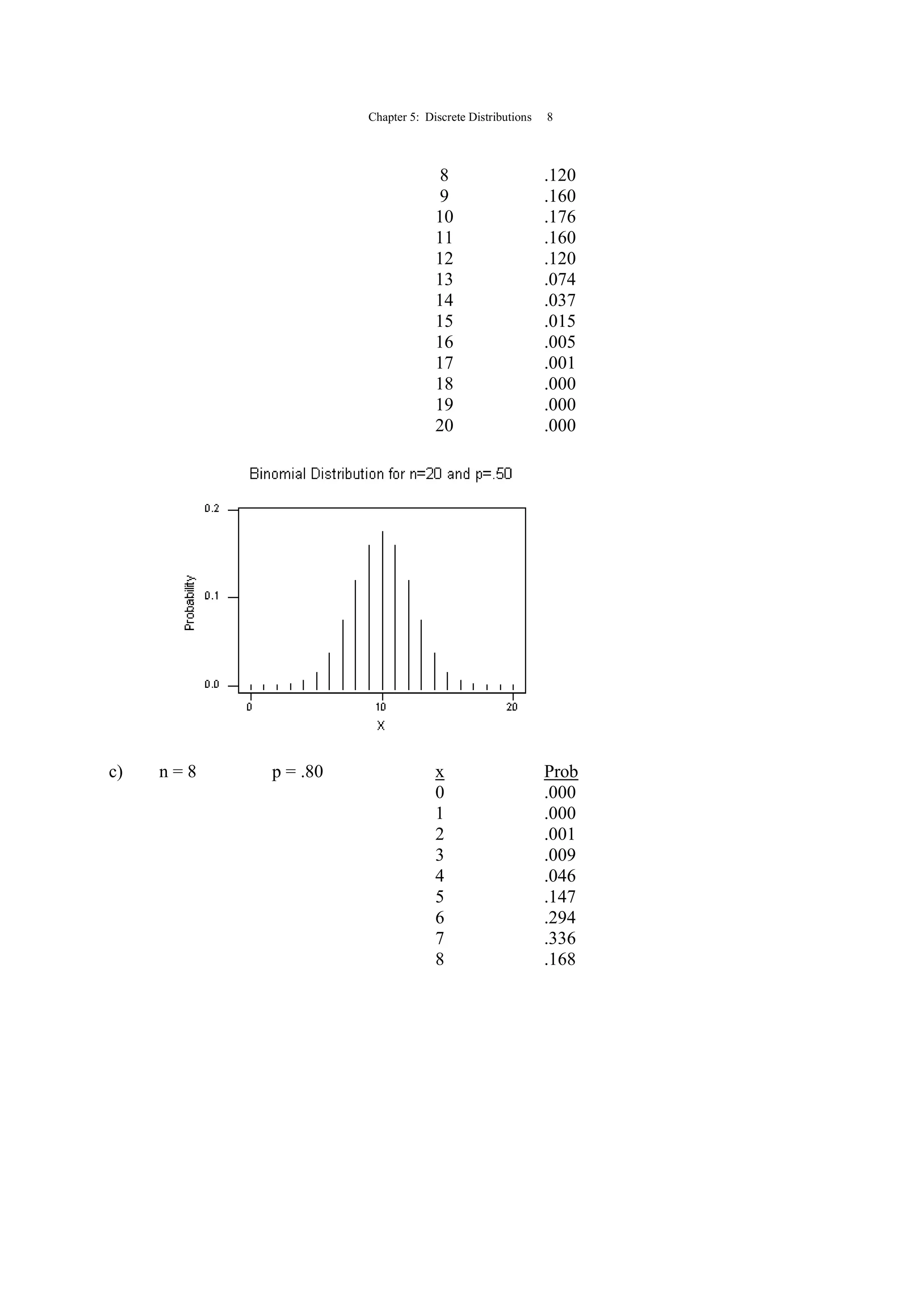
![Chapter 5: Discrete Distributions 3
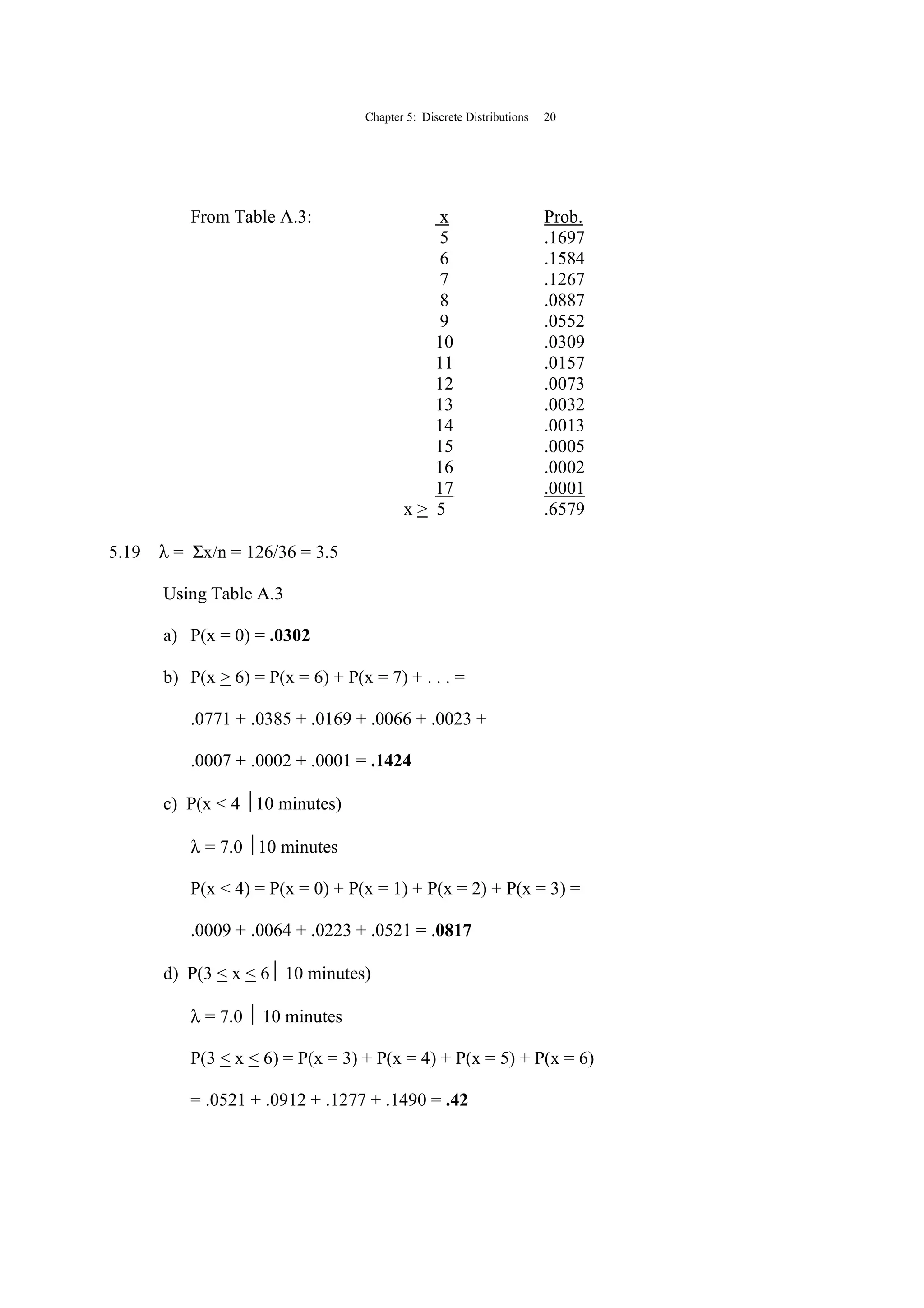
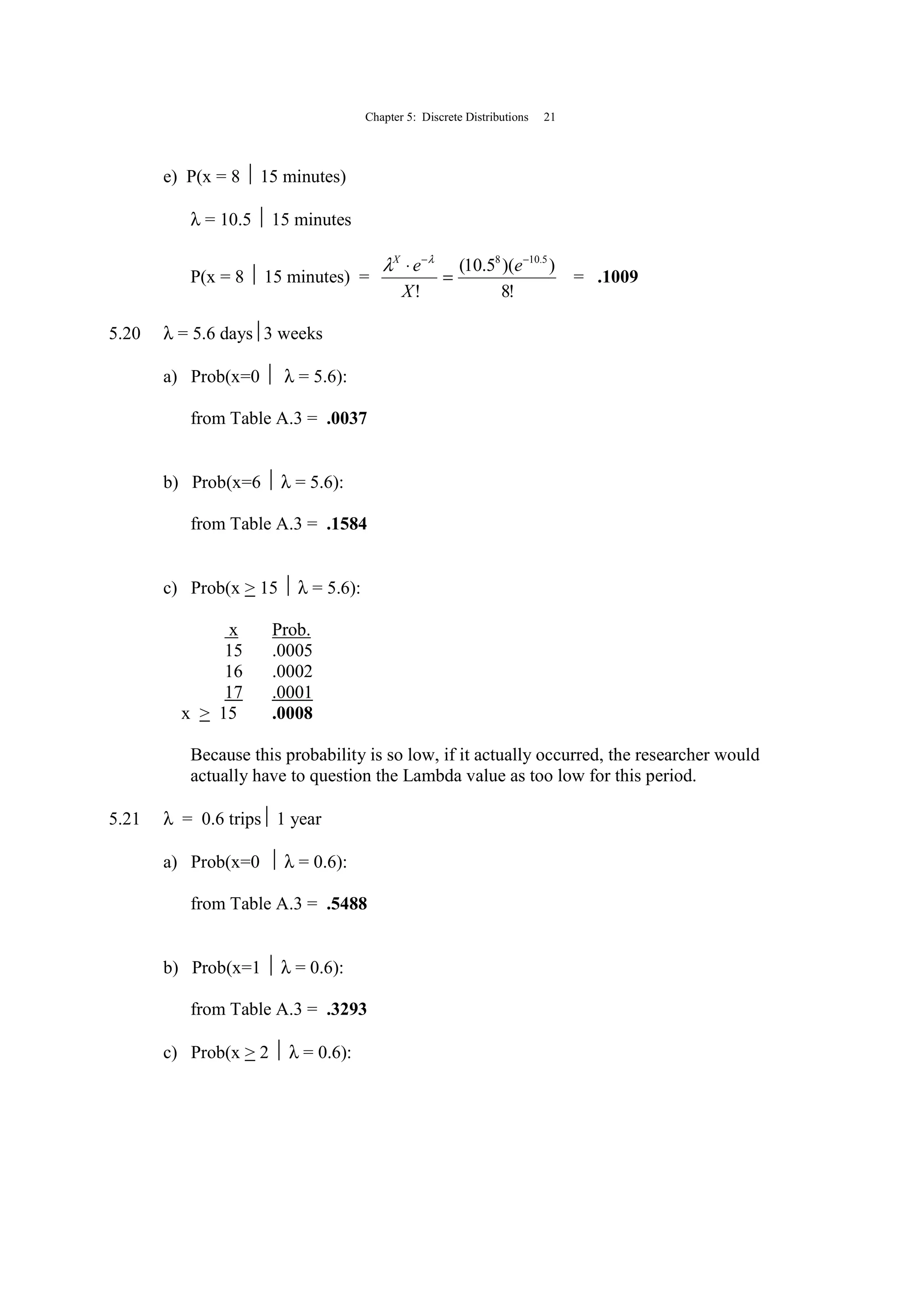
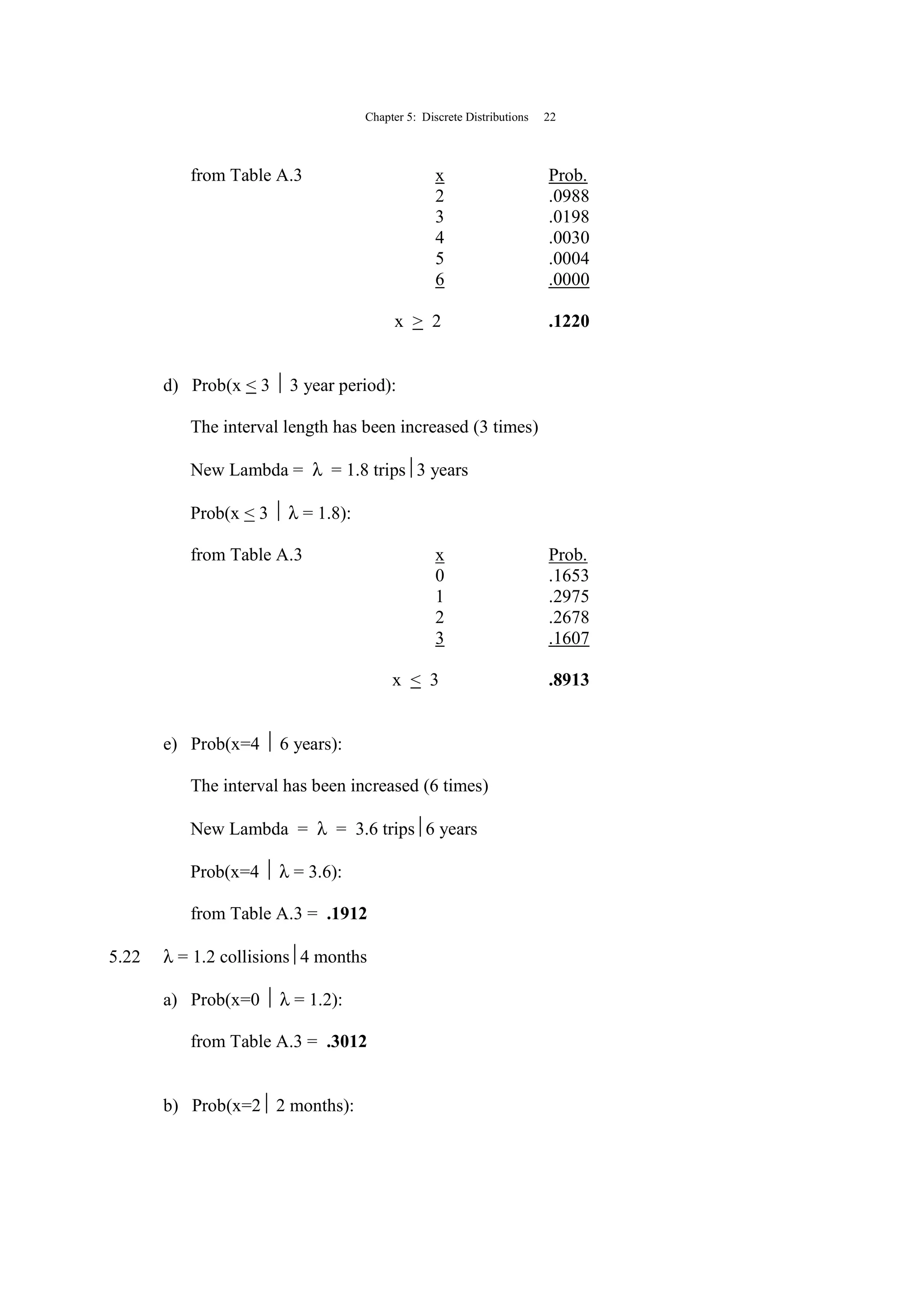
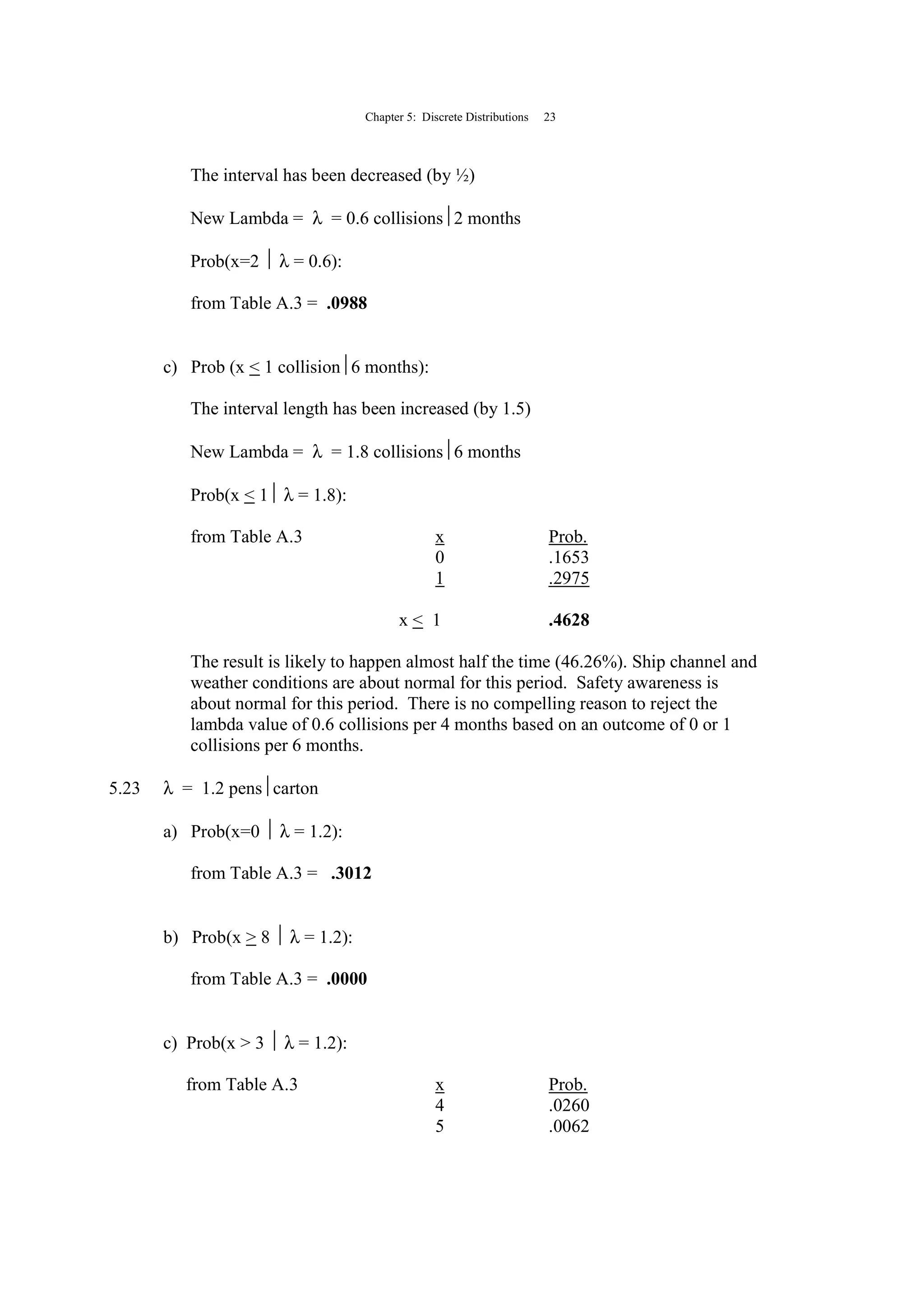
5.4 Poisson Distribution
Working Poisson Problems by Formula
Using the Poisson Tables
Mean and Standard Deviation of a Poisson Distribution
Graphing Poisson Distributions
Using the Computer to Generate Poisson Distributions
Approximating Binomial Problems by the Poisson Distribution
5.5 Hypergeometric Distribution
Using the Computer to Solve for Hypergeometric Distribution
Probabilities
KEY TERMS
Binomial Distribution Hypergeometric Distribution
Continuous Distributions Lambda (λ)
Continuous Random Variables Mean, or Expected Value
Discrete Distributions Poisson Distribution
Discrete Random Variables Random Variable
SOLUTIONS TO PROBLEMS IN CHAPTER 5
5.1 x P(x) x·P(x) (x-µ)2
(x-µ)2
·P(x)
1 .238 .238 2.775556 0.6605823
2 .290 .580 0.443556 0.1286312
3 .177 .531 0.111556 0.0197454
4 .158 .632 1.779556 0.2811700
5 .137 .685 5.447556 0.7463152
µ = [x·P(x)] = 2.666 σ2
= (x-µ)2
·P(x) = 1.836444
σ = 836444.1 = 1.355155](https://image.slidesharecdn.com/05chkenblacksolution-130815162851-phpapp01/75/05-ch-ken-black-solution-3-2048.jpg)
![Chapter 5: Discrete Distributions 4
5.2 x P(x) x·P(x) (x-µ)2
(x-µ)2
·P(x)
0 .103 .000 7.573504 0.780071
1 .118 .118 3.069504 0.362201
2 .246 .492 0.565504 0.139114
3 .229 .687 0.061504 0.014084
4 .138 .552 1.557504 0.214936
5 .094 .470 5.053504 0.475029
6 .071 .426 10.549500 0.749015
7 .001 .007 18.045500 0.018046
µ = [x·P(x)] = 2.752 σ2
= (x-µ)2
·P(x) = 2.752496
σ = 752496.2 = 1.6591
5.3 x P(x) x·P(x) (x-µ)2
(x-µ)2
·P(x)
0 .461 .000 0.913936 0.421324
1 .285 .285 0.001936 0.000552
2 .129 .258 1.089936 0.140602
3 .087 .261 4.177936 0.363480
4 .038 .152 9.265936 0.352106
E(x)=µ= [x·P(x)]= 0.956 σ2
= (x-µ)2
·P(x) = 1.278064
σ = 278064.1 = 1.1305
5.4 x P(x) x·P(x) (x-µ)2
(x-µ)2
·P(x)
0 .262 .000 1.4424 0.37791
1 .393 .393 0.0404 0.01588
2 .246 .492 0.6384 0.15705
3 .082 .246 3.2364 0.26538
4 .015 .060 7.8344 0.11752
5 .002 .010 14.4324 0.02886
6 .000 .000 23.0304 0.00000
µ = [x·P(x)] = 1.201 σ2
= (x-µ)2
·P(x) = 0.96260
σ = 96260. = .98112](https://image.slidesharecdn.com/05chkenblacksolution-130815162851-phpapp01/75/05-ch-ken-black-solution-4-2048.jpg)

This document provides an outline and learning objectives for Chapter 5 of a statistics textbook on discrete distributions. The chapter will: 1. Distinguish between discrete and continuous random variables and distributions. 2. Explain how to calculate the mean and variance of discrete distributions. 3. Cover the binomial distribution and how to solve problems using it. 4. Cover the Poisson distribution and how to solve problems using it. 5. Explain how to approximate binomial problems with the Poisson distribution. 6. Cover the hypergeometric distribution and how to solve problems using it.