This document discusses sampling distributions and their properties. It defines key terms like parameter, statistic, sampling variability, and sampling distribution. It explains that sampling distributions describe the distribution of all possible sample statistics from repeated sampling. The document then discusses sampling distributions for proportions and means specifically. It provides the formulas for the standard deviation of the sampling distribution and conditions for using the normal approximation. An example problem demonstrates how to calculate the probability of a sample proportion being more than 2% from the population parameter using the normal approximation.

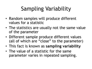
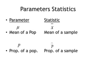
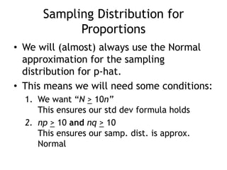
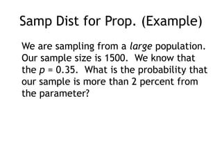
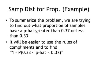
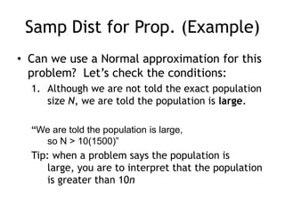
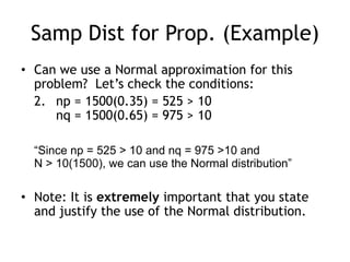
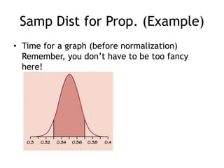
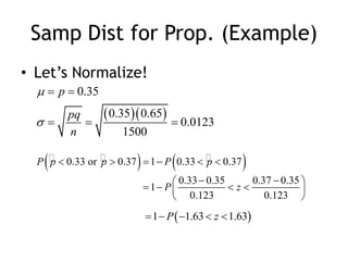
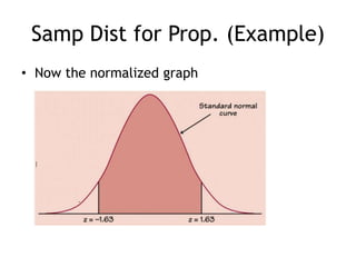
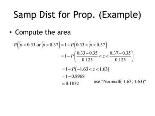
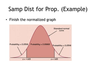
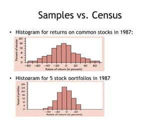
1. Chapter 9Sampling Distributions

2. 9.1 Sampling Distributions

3. DefinitionsParameterthe value of a characteristic for the entire population attained through censusin practice, is usually an unknown or estimated value

4. DefinitionsStatisticthe value of a characteristic for the entire population attained through samplingIn practice, the value of a statistic is used to estimate the parameter

5. Sampling VariabilityRandom samples will produce different values for a statisticThe statistics are usually not the same value of the parameterDifferent sample produce different values (all of which are “close” to the parameter)This fact is known as sampling variabilityThe value of a statistic for the same parameter varies in repeated sampling.

6. Parameters StatisticsParameterStatisticMean of a Pop Mean of a sampleProp. of a pop. Prop. of a sample

7. Sampling DistributionAll samples of size n are taken from a population of size NA histogram of these sample statistics is createdThis distribution is called the “sampling distribution”In practice, the sampling distribution is theorized, but never “created”

8. Creating a Sampling DistributionLet’s look at a pop N = 5, who answered ‘yes’ or ‘no’ to the question “Do you like toast?”We want to know proportion who say ‘yes’Here are the responses:ID Response01 Yes 02 No 03 Yes 04 No05 Yes

9. Creating a Sampling DistributionLet’s look at each sample and the phatfor sample size n = 3Sample #ID’s in samplep-hat1 01, 02, 03 0.662 01, 02, 04 0.333 01, 02, 05 0.664 01, 03, 04 0.665 01, 03, 05 16 01, 04, 05 0.667 02, 03, 04 0.338 02, 03, 05 0.669 02, 04, 05 0.3310 03, 04, 05 0.66You can imagine that this quickly gets labor intensive!

10. Creating a Sampling DistributionCreate a HistogramClass Count0.00-0.24 00.25-0.49 30.50-0.74 60.75-1.00 1Notice that p = 0.6, and the mean of this distribution is approx 0.676543210 0.5 1

11. Describing Sampling DistributionsLike most 1-var data, we describe :CenterShapeSpreadUnusual features/OutliersIf you are using a sample to estimate a parameter, of the sampling distribution:Where should the center be?What about the “ideal shape?”What would you like the spread to be?Would outliers be helpful?

12. Sampling Distribution and BiasWhen a statistic is unbiased, the mean of the sampling distribution is the value of the parameter.This is actually a pretty powerful statement. In order to find the value of the parameter, you just need to take a lot of samples! (wait, that’s not good either)Revision: If a statistic is unbiased, then “chances are” the value of any sample should be close to the value of parameterStatistics that are unbiased are called “unbiased estimators” (these are good)

13. Variability of a StatisticThe spread of a sampling distribution is known as the variability of the statisticLarge sample size = less variability

14. The Enemies of SamplingEnemy #1: BiasEnemy #2: VariabilityA visual of the difference:

15. The Enemies of SamplingAnother look with Histograms:

16. 9.2 Sample Proportions

17. Sampling Distribution for ProportionsFor each sample, calculate p-hat:The sampling distribution of p-hat will have:Mean = p (the parameter)Standard deviation:

18. Sampling Distribution for ProportionsNotice that this is an unbiased estimator!The standard deviation decreases when the sample size is largeStd. Dev. and sample size have an “inverse square” relationEx. If we want ½ the std dev, we need to 4x the sample sizeEx. If we want to 1/3 the std dev,we need to 9x the sample size

19. Sampling Distribution for ProportionsWe will (almost) always use the Normal approximation for the sampling distribution for p-hat.This means we will need some conditions:We want “N> 10n”This ensures our std dev formula holdsnp> 10 andnq> 10This ensures our samp. dist. is approx. Normal

20. Samp Dist for Prop. (Example) We are sampling from a large population. Our sample size is 1500. We know that the p = 0.35. What is the probability that our sample is more than 2 percent from the parameter?

21. Samp Dist for Prop. (Example)To summarize the problem, we are trying to find out what proportion of samples have a p-hat greater than 0.37 or less than 0.33It will be easier to use the rules of compliments and to find “1 – P(0.33 < p-hat < 0.37)”

22. Samp Dist for Prop. (Example)Can we use a Normal approximation for this problem? Let’s check the conditions:Although we are not told the exact population size N, we are told the population is large.“We are told the population is large, so N > 10(1500)” Tip: when a problem says the population is large, you are to interpret that the population is greater than 10n

23. Samp Dist for Prop. (Example)Can we use a Normal approximation for this problem? Let’s check the conditions: 2. np = 1500(0.35) = 525 > 10nq = 1500(0.65) = 975 > 10“Since np = 525 > 10 and nq = 975 >10 and N > 10(1500), we can use the Normal distribution”Note: It is extremely important that you state and justify the use of the Normal distribution.

24. Samp Dist for Prop. (Example)Time for a graph (before normalization)Remember, you don’t have to be too fancy here!

25. Samp Dist for Prop. (Example)Let’s Normalize!

26. Samp Dist for Prop. (Example)Now the normalized graph

27. Samp Dist for Prop. (Example)Compute the area

28. Samp Dist for Prop. (Example)Finish the normalized graph

29. Samp Dist for Prop. (Example)Summary:“The probability that a sample (n=1500) is more than 2 percent from the parameter is 0.1032”Notes: remember that in this context, probability is the same as proportion, and proportion is the same as area.Actually, you’ve done many of these kinds of problems already, right?

30. 9.3 Sample Means

31. Samples vs. CensusHistogram for returns on common stocks in 1987:Histogram for 5 stock portfolios in 1987

32. Samples vs. CensusWe can see from the previous slide that the distribution of samples (portfolio)Are less variable than the censusAre more Normal than the census

33. Sampling Distribution for MeansSuppose we have a sampling distribution of samples size n from a large populationThe mean of the sampling distribution is the mean of the populationThe std dev of the samp dist is given by:

34. Sampling Distribution for MeansThe sample mean is an unbiased estimator of the population meanLike for proportions, the std dev and the population size have an inverse square relationLike for proportions, we need N> 10n for our std dev formula to hold upThis sampling distribution holds true even if the population is not Normal!

35. The Central Limit TheoremAn SRS of size n from any population will produce a sampling distribution that is N( , /(n)) whenever n is large enough.Caution: this theorem is only true for means. Do not try to use the CLT for proportions!

36. The Central Limit TheoremWhy we use CLT:From the previous section, we saw that we use the Normal dist to gauge probability of producing samplesWe invoke the CLT to justify usage of the Normal distributionUsing Normal dist w/o justification is a “nono”

37. The Central Limit TheoremWhen to use the CLT:Sampling Distribution for a mean ()We need to Normalize the sample meanThe sample is described as “large”Generally, n> 30The raw data is not given