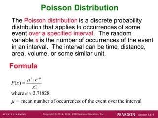
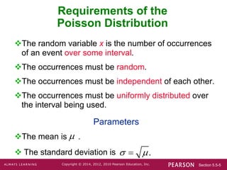
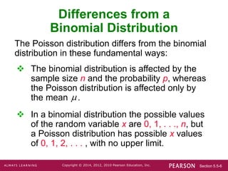
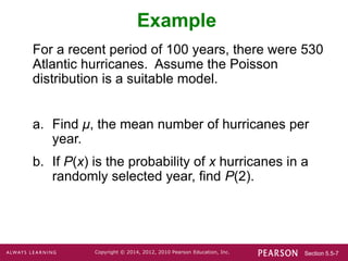
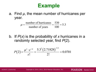
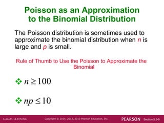
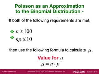
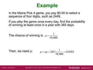
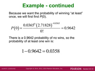
Section 5.5-1
Copyright © 2014, 2012, 2010 Pearson Education, Inc.
Lecture Slides
Elementary Statistics
Twelfth Edition
and the Triola Statistics Series
by Mario F. Triola
Section 5.5-2
Copyright © 2014, 2012, 2010 Pearson Education, Inc.
Chapter 5
Probability Distributions
5-1 Review and Preview
5-2 Probability Distributions
5-3 Binomial Probability Distributions
5-4 Parameters for Binomial Distributions
5-5 Poisson Probability Distributions
Section 5.5-3
Copyright © 2014, 2012, 2010 Pearson Education, Inc.
Key Concept
The Poisson distribution is another
discrete probability distribution which is
important because it is often used for
describing the behavior of rare events
(with small probabilities).
Section 5.5-4
Copyright © 2014, 2012, 2010 Pearson Education, Inc.
Poisson Distribution
The Poisson distribution is a discrete probability
distribution that applies to occurrences of some
event over a specified interval. The random
variable x is the number of occurrences of the event
in an interval. The interval can be time, distance,
area, volume, or some similar unit.
Formula
( )
!
where 2.71828
mean number of occurrences of the event over the interval
x
e
P x
x
e








Section 5.5-5
Copyright © 2014, 2012, 2010 Pearson Education, Inc.
Requirements of the
Poisson Distribution
The random variable x is the number of occurrences
of an event over some interval.
The occurrences must be random.
The occurrences must be independent of each other.
The occurrences must be uniformly distributed over
the interval being used.
Parameters
The mean is .
 The standard deviation is

.
 

Section 5.5-6
Copyright © 2014, 2012, 2010 Pearson Education, Inc.
Differences from a
Binomial Distribution
The Poisson distribution differs from the binomial
distribution in these fundamental ways:
 The binomial distribution is affected by the
sample size n and the probability p, whereas
the Poisson distribution is affected only by
the mean .
 In a binomial distribution the possible values
of the random variable x are 0, 1, . . ., n, but
a Poisson distribution has possible x values
of 0, 1, 2, . . . , with no upper limit.

Section 5.5-7
Copyright © 2014, 2012, 2010 Pearson Education, Inc.
Example
For a recent period of 100 years, there were 530
Atlantic hurricanes. Assume the Poisson
distribution is a suitable model.
a. Find μ, the mean number of hurricanes per
year.
b. If P(x) is the probability of x hurricanes in a
randomly selected year, find P(2).
Section 5.5-8
Copyright © 2014, 2012, 2010 Pearson Education, Inc.
Example
a. Find μ, the mean number of hurricanes per
year.
b. If P(x) is the probability of x hurricanes in a
randomly selected year, find P(2).
number of hurricanes 530
5.3
number of years 100
   
 
 
5.3
2
5.3 2.71828
2 0.0701
! 2!
x
e
P
x





  
Section 5.5-9
Copyright © 2014, 2012, 2010 Pearson Education, Inc.
Poisson as an Approximation
to the Binomial Distribution
Rule of Thumb to Use the Poisson to Approximate the
Binomial


The Poisson distribution is sometimes used to
approximate the binomial distribution when n is
large and p is small.
100
n 
10
np 
Section 5.5-10
Copyright © 2014, 2012, 2010 Pearson Education, Inc.
Poisson as an Approximation
to the Binomial Distribution -
Value for


If both of the following requirements are met,
then use the following formula to calculate ,
100
n 
10
np 


n p
  
Section 5.5-11
Copyright © 2014, 2012, 2010 Pearson Education, Inc.
Example
In the Maine Pick 4 game, you pay $0.50 to select a
sequence of four digits, such as 2449.
If you play the game once every day, find the probability
of winning at least once in a year with 365 days.
The chance of winning is
Then, we need μ: 1
365 0.0365
10,000
np
   
1
10,000
p 
Section 5.5-12
Copyright © 2014, 2012, 2010 Pearson Education, Inc.
Example - continued
Because we want the probability of winning “at least”
once, we will first find P(0).
There is a 0.9642 probability of no wins, so the
probability of at least one win is:
 
 
0.0365
0
0.0365 2.71828
0 0.9642
0!
P

 
1 0.9642 0.0358
 

Chapter 5 Section (5).ppt

  • 1.
    Section 5.5-1 Copyright ©2014, 2012, 2010 Pearson Education, Inc. Lecture Slides Elementary Statistics Twelfth Edition and the Triola Statistics Series by Mario F. Triola
  • 2.
    Section 5.5-2 Copyright ©2014, 2012, 2010 Pearson Education, Inc. Chapter 5 Probability Distributions 5-1 Review and Preview 5-2 Probability Distributions 5-3 Binomial Probability Distributions 5-4 Parameters for Binomial Distributions 5-5 Poisson Probability Distributions
  • 3.
    Section 5.5-3 Copyright ©2014, 2012, 2010 Pearson Education, Inc. Key Concept The Poisson distribution is another discrete probability distribution which is important because it is often used for describing the behavior of rare events (with small probabilities).
  • 4.
    Section 5.5-4 Copyright ©2014, 2012, 2010 Pearson Education, Inc. Poisson Distribution The Poisson distribution is a discrete probability distribution that applies to occurrences of some event over a specified interval. The random variable x is the number of occurrences of the event in an interval. The interval can be time, distance, area, volume, or some similar unit. Formula ( ) ! where 2.71828 mean number of occurrences of the event over the interval x e P x x e        
  • 5.
    Section 5.5-5 Copyright ©2014, 2012, 2010 Pearson Education, Inc. Requirements of the Poisson Distribution The random variable x is the number of occurrences of an event over some interval. The occurrences must be random. The occurrences must be independent of each other. The occurrences must be uniformly distributed over the interval being used. Parameters The mean is .  The standard deviation is  .   
  • 6.
    Section 5.5-6 Copyright ©2014, 2012, 2010 Pearson Education, Inc. Differences from a Binomial Distribution The Poisson distribution differs from the binomial distribution in these fundamental ways:  The binomial distribution is affected by the sample size n and the probability p, whereas the Poisson distribution is affected only by the mean .  In a binomial distribution the possible values of the random variable x are 0, 1, . . ., n, but a Poisson distribution has possible x values of 0, 1, 2, . . . , with no upper limit. 
  • 7.
    Section 5.5-7 Copyright ©2014, 2012, 2010 Pearson Education, Inc. Example For a recent period of 100 years, there were 530 Atlantic hurricanes. Assume the Poisson distribution is a suitable model. a. Find μ, the mean number of hurricanes per year. b. If P(x) is the probability of x hurricanes in a randomly selected year, find P(2).
  • 8.
    Section 5.5-8 Copyright ©2014, 2012, 2010 Pearson Education, Inc. Example a. Find μ, the mean number of hurricanes per year. b. If P(x) is the probability of x hurricanes in a randomly selected year, find P(2). number of hurricanes 530 5.3 number of years 100         5.3 2 5.3 2.71828 2 0.0701 ! 2! x e P x        
  • 9.
    Section 5.5-9 Copyright ©2014, 2012, 2010 Pearson Education, Inc. Poisson as an Approximation to the Binomial Distribution Rule of Thumb to Use the Poisson to Approximate the Binomial   The Poisson distribution is sometimes used to approximate the binomial distribution when n is large and p is small. 100 n  10 np 
  • 10.
    Section 5.5-10 Copyright ©2014, 2012, 2010 Pearson Education, Inc. Poisson as an Approximation to the Binomial Distribution - Value for   If both of the following requirements are met, then use the following formula to calculate , 100 n  10 np    n p   
  • 11.
    Section 5.5-11 Copyright ©2014, 2012, 2010 Pearson Education, Inc. Example In the Maine Pick 4 game, you pay $0.50 to select a sequence of four digits, such as 2449. If you play the game once every day, find the probability of winning at least once in a year with 365 days. The chance of winning is Then, we need μ: 1 365 0.0365 10,000 np     1 10,000 p 
  • 12.
    Section 5.5-12 Copyright ©2014, 2012, 2010 Pearson Education, Inc. Example - continued Because we want the probability of winning “at least” once, we will first find P(0). There is a 0.9642 probability of no wins, so the probability of at least one win is:     0.0365 0 0.0365 2.71828 0 0.9642 0! P    1 0.9642 0.0358  