Chapter 3 Section 4.ppt

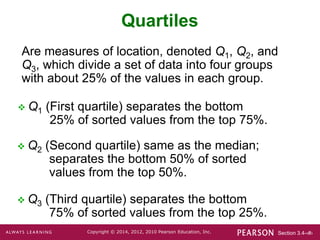
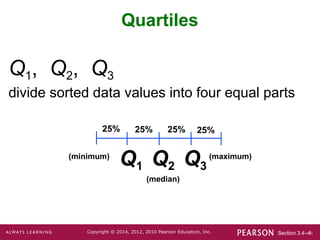
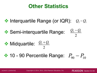
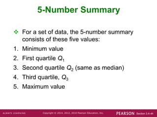
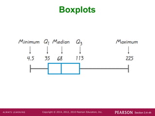
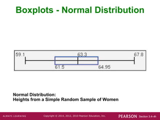
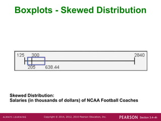
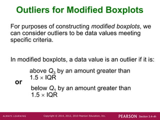
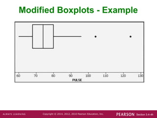
Section 3.4-‹#›
Copyright © 2014, 2012, 2010 Pearson Education, Inc.
Lecture Slides
Elementary Statistics
Twelfth Edition
and the Triola Statistics Series
by Mario F. Triola

Section 3.4-‹#›
Chapter 3
Statistics for Describing,
Exploring, and Comparing Data
3-1 Review and Preview
3-2 Measures of Center
3-3 Measures of Variation
3-4 Measures of Relative Standing and
Boxplots

Section 3.4-‹#›
Key Concept
This section introduces measures of relative
standing, which are numbers showing the
location of data values relative to the other values
within a data set.
They can be used to compare values from
different data sets, or to compare values within
the same data set.
The most important concept is the z score.
We will also discuss percentiles and quartiles, as
well as a new statistical graph called the boxplot.

Section 3.4-‹#›
Basics of z Scores,
Percentiles, Quartiles, and
Boxplots
Part 1

Section 3.4-‹#›
 z Score (or standardized value)
the number of standard deviations that a given
value x is above or below the mean
z score

Section 3.4-‹#›
Sample
x x
z
s


Population
Round z scores to 2 decimal places
Measures of Position z Score
x
z





Section 3.4-‹#›
Interpreting Z Scores
Whenever a value is less than the mean, its
corresponding z score is negative
Ordinary values:
Unusual Values:
2 score 2
z
  
score 2 or score 2
z z
  

Section 3.4-‹#›
Example
The author of the text measured his pulse rate to
be 48 beats per minute.
Is that pulse rate unusual if the mean adult male
pulse rate is 67.3 beats per minute with a
standard deviation of 10.3?
Answer: Since the z score is between – 2 and +2,
his pulse rate is not unusual.
48 67.3
1.87
10.3
x x
z
s
 
   

Section 3.4-‹#›
Percentiles
are measures of location. There are 99
percentiles denoted P1, P2, . . ., P99, which
divide a set of data into 100 groups with
about 1% of the values in each group.

Section 3.4-‹#›
Finding the Percentile
of a Data Value
Percentile of value x = • 100
number of values less than x
total number of values

Section 3.4-‹#›
Example
For the 40 Chips Ahoy cookies, find the percentile for a cookie with
23 chips.
Answer: We see there are 10 cookies with fewer than 23 chips, so
A cookie with 23 chips is in the 25th percentile.
10
Percentile of 23 100 25
40
 

Section 3.4-‹#›
n total number of values in the
data set
k percentile being used
L locator that gives the position of
a value
Pk kth percentile
Notation
Converting from the kth Percentile to
the Corresponding Data Value
100
k
L n
 

Section 3.4-‹#›
Converting from the
kth Percentile to the
Corresponding Data Value

Section 3.4-‹#›
Quartiles
 Q1 (First quartile) separates the bottom
25% of sorted values from the top 75%.
 Q2 (Second quartile) same as the median;
separates the bottom 50% of sorted
values from the top 50%.
 Q3 (Third quartile) separates the bottom
75% of sorted values from the top 25%.
Are measures of location, denoted Q1, Q2, and
Q3, which divide a set of data into four groups
with about 25% of the values in each group.

Section 3.4-‹#›
Q1, Q2, Q3
divide sorted data values into four equal parts
Quartiles
25% 25% 25% 25%
Q3
Q2
Q1
(minimum) (maximum)
(median)

Section 3.4-‹#›
Other Statistics
 Interquartile Range (or IQR):
 10 - 90 Percentile Range:
 Midquartile:
 Semi-interquartile Range: 3 1
2
Q Q

3 1
Q Q

3 1
2
Q Q

90 10
P P


Section 3.4-‹#›
 For a set of data, the 5-number summary
consists of these five values:
1. Minimum value
2. First quartile Q1
3. Second quartile Q2 (same as median)
4. Third quartile, Q3
5. Maximum value
5-Number Summary

Section 3.4-‹#›
 A boxplot (or box-and-whisker-diagram) is a
graph of a data set that consists of a line
extending from the minimum value to the
maximum value, and a box with lines drawn
at the first quartile, Q1, the median, and the
third quartile, Q3.
Boxplot

Section 3.4-‹#›
1. Find the 5-number summary.
2. Construct a scale with values that include
the minimum and maximum data values.
3. Construct a box (rectangle) extending from
Q1 to Q3 and draw a line in the box at the
value of Q2 (median).
4. Draw lines extending outward from the box
to the minimum and maximum values.
Boxplot - Construction

Section 3.4-‹#›
Boxplots

Section 3.4-‹#›
Boxplots - Normal Distribution
Normal Distribution:
Heights from a Simple Random Sample of Women

Section 3.4-‹#›
Boxplots - Skewed Distribution
Skewed Distribution:
Salaries (in thousands of dollars) of NCAA Football Coaches

Section 3.4-‹#›
Outliers and
Modified Boxplots
Part 2

Section 3.4-‹#›
Outliers
 An outlier is a value that lies very far away
from the vast majority of the other values
in a data set.

Section 3.4-‹#›
Important Principles
 An outlier can have a dramatic effect on the
mean and the standard deviation.
 An outlier can have a dramatic effect on the
scale of the histogram so that the true nature of
the distribution is totally obscured.

Section 3.4-‹#›
Outliers for Modified Boxplots
For purposes of constructing modified boxplots, we
can consider outliers to be data values meeting
specific criteria.
In modified boxplots, a data value is an outlier if it is:
above Q3 by an amount greater than
1.5  IQR
below Q1 by an amount greater than
1.5  IQR
or

Section 3.4-‹#›
Modified Boxplots
Boxplots described earlier are called skeletal (or
regular) boxplots.
Some statistical packages provide modified
boxplots which represent outliers as special
points.

Section 3.4-‹#›
Modified Boxplot Construction
 A special symbol (such as an asterisk) is
used to identify outliers.
 The solid horizontal line extends only as far
as the minimum data value that is not an
outlier and the maximum data value that is
not an outlier.
A modified boxplot is constructed with these
specifications:

Section 3.4-‹#›
Modified Boxplots - Example

Section 3.4-‹#›
Putting It All Together
 So far, we have discussed several basic tools
commonly used in statistics –
 Context of data
 Source of data
 Sampling method
 Measures of center and variation
 Distribution and outliers
 Changing patterns over time
 Conclusions and practical implications
 This is an excellent checklist, but it should not
replace thinking about any other relevant factors.

Chapter 3 Section 4.ppt

More Related Content

Similar to Chapter 3 Section 4.ppt

More from ManoloTaquire

Recently uploaded

Chapter 3 Section 4.ppt