Chapter 3 Section 3.ppt

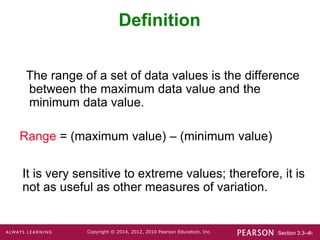
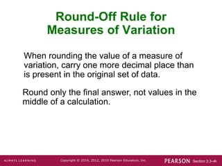
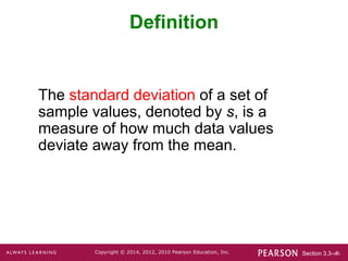
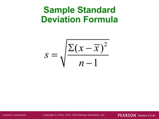
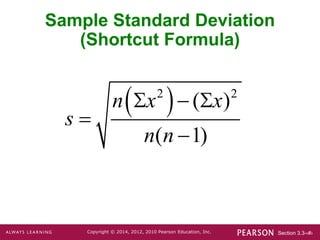
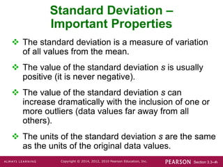
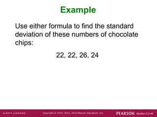
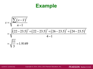
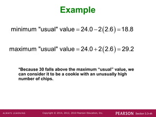
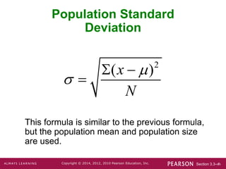
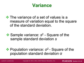
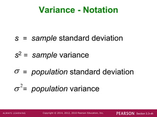
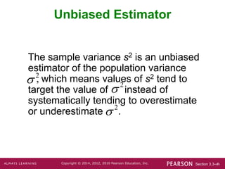
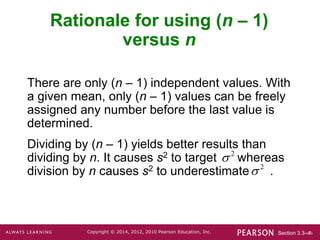
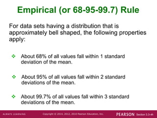
Section 3.3-‹#›
Copyright © 2014, 2012, 2010 Pearson Education, Inc.
Lecture Slides
Elementary Statistics
Twelfth Edition
and the Triola Statistics Series
by Mario F. Triola

Section 3.3-‹#›
Chapter 3
Statistics for Describing,
Exploring, and Comparing Data
3-1 Review and Preview
3-2 Measures of Center
3-3 Measures of Variation
3-4 Measures of Relative Standing and
Boxplots

Section 3.3-‹#›
Key Concept
Discuss characteristics of variation, in particular,
measures of variation, such as standard deviation,
for analyzing data.
Make understanding and interpreting the standard
deviation a priority.

Section 3.3-‹#›
Basics Concepts of Variation
Part 1

Section 3.3-‹#›
Definition
The range of a set of data values is the difference
between the maximum data value and the
minimum data value.
Range = (maximum value) – (minimum value)
It is very sensitive to extreme values; therefore, it is
not as useful as other measures of variation.

Section 3.3-‹#›
Round-Off Rule for
Measures of Variation
When rounding the value of a measure of
variation, carry one more decimal place than
is present in the original set of data.
Round only the final answer, not values in the
middle of a calculation.

Section 3.3-‹#›
Definition
The standard deviation of a set of
sample values, denoted by s, is a
measure of how much data values
deviate away from the mean.

Section 3.3-‹#›
Sample Standard
Deviation Formula
2
( )
1
x x
s
n
 



Section 3.3-‹#›
Sample Standard Deviation
(Shortcut Formula)
 
2 2
( )
( 1)
n x x
s
n n
  



Section 3.3-‹#›
Standard Deviation –
Important Properties
 The standard deviation is a measure of variation
of all values from the mean.
 The value of the standard deviation s is usually
positive (it is never negative).
 The value of the standard deviation s can
increase dramatically with the inclusion of one or
more outliers (data values far away from all
others).
 The units of the standard deviation s are the same
as the units of the original data values.

Section 3.3-‹#›
Example
Use either formula to find the standard
deviation of these numbers of chocolate
chips:
22, 22, 26, 24

Section 3.3-‹#›
Example
 
       
2
2 2 2 2
1
22 23.5 22 23.5 26 23.5 24 23.5
4 1
11
1.9149
3
x x
s
n



      


 


Section 3.3-‹#›
Range Rule of Thumb for
Understanding Standard Deviation
It is based on the principle that for many
data sets, the vast majority (such as
95%) of sample values lie within two
standard deviations of the mean.

Section 3.3-‹#›
Interpreting a Known Value of the
Standard Deviation
Informally define usual values in a data set to be
those that are typical and not too extreme. Find
rough estimates of the minimum and maximum
“usual” sample values as follows:
Minimum “usual” value (mean) – 2  (standard deviation)
=
Maximum “usual” value (mean) + 2  (standard deviation)
=

Section 3.3-‹#›
Estimating a Value of the
Standard Deviation s
To roughly estimate the standard deviation from
a collection of known sample data use
where
range = (maximum value) – (minimum value)

4
range
s

Section 3.3-‹#›
Example
Using the 40 chocolate chip counts for the
Chips Ahoy cookies, the mean is 24.0 chips
and the standard deviation is 2.6 chips.
Use the range rule of thumb to find the
minimum and maximum “usual” numbers of
chips.
Would a cookie with 30 chocolate chips be
“unusual”?

Section 3.3-‹#›
Example
 
 
. . .
. . .
  
  
minimum "usual" value 24 0 2 2 6 18 8
maximum "usual" value 24 0 2 2 6 29 2
*Because 30 falls above the maximum “usual” value, we
can consider it to be a cookie with an unusually high
number of chips.

Section 3.3-‹#›
Comparing Variation in
Different Samples
It’s a good practice to compare two sample
standard deviations only when the sample
means are approximately the same.
When comparing variation in samples with very
different means, it is better to use the coefficient
of variation, which is defined later in this section.

Section 3.3-‹#›
Population Standard
Deviation
This formula is similar to the previous formula,
but the population mean and population size
are used.
2
( )
x
N


 


Section 3.3-‹#›
Variance
 Population variance: σ2 - Square of the
population standard deviation σ
 The variance of a set of values is a
measure of variation equal to the square
of the standard deviation.
 Sample variance: s2 - Square of the
sample standard deviation s

Section 3.3-‹#›
Variance - Notation
s = sample standard deviation
s2 = sample variance
= population standard deviation
= population variance
2



Section 3.3-‹#›
Unbiased Estimator
The sample variance s2 is an unbiased
estimator of the population variance
, which means values of s2 tend to
target the value of instead of
systematically tending to overestimate
or underestimate .
2
 2

2


Section 3.3-‹#›
Beyond the Basics of
Variation
Part 2

Section 3.3-‹#›
Rationale for using (n – 1)
versus n
There are only (n – 1) independent values. With
a given mean, only (n – 1) values can be freely
assigned any number before the last value is
determined.
Dividing by (n – 1) yields better results than
dividing by n. It causes s2 to target whereas
division by n causes s2 to underestimate .
2

2


Section 3.3-‹#›
Empirical (or 68-95-99.7) Rule
For data sets having a distribution that is
approximately bell shaped, the following properties
apply:
 About 68% of all values fall within 1 standard
deviation of the mean.
 About 95% of all values fall within 2 standard
deviations of the mean.
 About 99.7% of all values fall within 3 standard
deviations of the mean.

Section 3.3-‹#›
The Empirical Rule

Section 3.3-‹#›
Chebyshev’s Theorem
The proportion (or fraction) of any set of data
lying within K standard deviations of the mean is
always at least 1–1/K2, where K is any positive
number greater than 1.
 For K = 2, at least 3/4 (or 75%) of all values
lie within 2 standard deviations of the mean.
 For K = 3, at least 8/9 (or 89%) of all values
lie within 3 standard deviations of the mean.

Section 3.3-‹#›
Example
IQ scores have a mean of 100 and a standard
deviation of 15. What can we conclude from
Chebyshev’s theorem?
•At least 75% of IQ scores are within 2 standard
deviations of 100, or between 70 and 130.
•At least 88.9% of IQ scores are within 3 standard
deviations of 100, or between 55 and 145.

Section 3.3-‹#›
Coefficient of Variation
The coefficient of variation (or CV) for a set of
nonnegative sample or population data,
expressed as a percent, describes the
standard deviation relative to the mean.
Sample Population
100%
s
cv
x
  100%
cv


 

Chapter 3 Section 3.ppt

More Related Content

Similar to Chapter 3 Section 3.ppt

More from ManoloTaquire

Recently uploaded

Chapter 3 Section 3.ppt