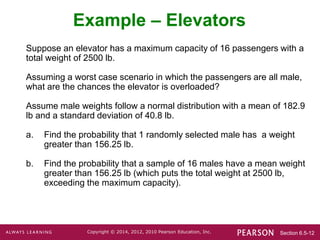
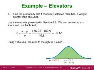
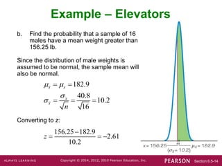
Section 6.5-1
Copyright © 2014, 2012, 2010 Pearson Education, Inc.
Lecture Slides
Elementary Statistics
Twelfth Edition
and the Triola Statistics Series
by Mario F. Triola
Section 6.5-2
Copyright © 2014, 2012, 2010 Pearson Education, Inc.
Chapter 6
Normal Probability Distributions
6-1 Review and Preview
6-2 The Standard Normal Distribution
6-3 Applications of Normal Distributions
6-4 Sampling Distributions and Estimators
6-5 The Central Limit Theorem
6-6 Assessing Normality
6-7 Normal as Approximation to Binomial
Section 6.5-3
Copyright © 2014, 2012, 2010 Pearson Education, Inc.
Key Concept
The Central Limit Theorem tells us that for a
population with any distribution, the distribution of
the sample means approaches a normal
distribution as the sample size increases.
The procedure in this section forms the foundation
for estimating population parameters and
hypothesis testing.
Section 6.5-4
Copyright © 2014, 2012, 2010 Pearson Education, Inc.
Central Limit Theorem
1. The random variable x has a distribution (which may or
may not be normal) with mean μ and standard deviation σ.
2. Simple random samples all of size n are selected from the
population. (The samples are selected so that all possible
samples of the same size n have the same chance of
being selected.)
Given:
Section 6.5-5
Copyright © 2014, 2012, 2010 Pearson Education, Inc.
1. The distribution of sample will, as the
sample size increases, approach a normal
distribution.
2. The mean of the sample means is the
population mean .
3. The standard deviation of all sample means
is .
Conclusions:
Central Limit Theorem – cont.
x

/ n

Section 6.5-6
Copyright © 2014, 2012, 2010 Pearson Education, Inc.
Practical Rules Commonly Used
1. For samples of size n larger than 30, the distribution of
the sample means can be approximated reasonably well
by a normal distribution. The approximation becomes
closer to a normal distribution as the sample size n
becomes larger.
2. If the original population is normally distributed, then for
any sample size n, the sample means will be normally
distributed (not just the values of n larger than 30).
Section 6.5-7
Copyright © 2014, 2012, 2010 Pearson Education, Inc.
The mean of the sample means
The standard deviation of sample mean
(often called the standard error of the mean)
Notation
x
 

x
n

 
Section 6.5-8
Copyright © 2014, 2012, 2010 Pearson Education, Inc.
Example - Normal Distribution
As we proceed from
n = 1 to n = 50, we
see that the
distribution of
sample means is
approaching the
shape of a normal
distribution.
Section 6.5-9
Copyright © 2014, 2012, 2010 Pearson Education, Inc.
Example - Uniform Distribution
As we proceed from
n = 1 to n = 50, we
see that the
distribution of
sample means is
approaching the
shape of a normal
distribution.
Section 6.5-10
Copyright © 2014, 2012, 2010 Pearson Education, Inc.
Example - U-Shaped Distribution
As we proceed from
n = 1 to n = 50, we
see that the
distribution of
sample means is
approaching the
shape of a normal
distribution.
Section 6.5-11
Copyright © 2014, 2012, 2010 Pearson Education, Inc.
As the sample size increases, the
sampling distribution of sample
means approaches a normal
distribution.
Important Point
Section 6.5-12
Copyright © 2014, 2012, 2010 Pearson Education, Inc.
Suppose an elevator has a maximum capacity of 16 passengers with a
total weight of 2500 lb.
Assuming a worst case scenario in which the passengers are all male,
what are the chances the elevator is overloaded?
Assume male weights follow a normal distribution with a mean of 182.9
lb and a standard deviation of 40.8 lb.
a. Find the probability that 1 randomly selected male has a weight
greater than 156.25 lb.
b. Find the probability that a sample of 16 males have a mean weight
greater than 156.25 lb (which puts the total weight at 2500 lb,
exceeding the maximum capacity).
Example – Elevators
Section 6.5-13
Copyright © 2014, 2012, 2010 Pearson Education, Inc.
a. Find the probability that 1 randomly selected male has a weight
greater than 156.25 lb.
Use the methods presented in Section 6.3. We can convert to a z
score and use Table A-2.
Using Table A-2, the area to the right is 0.7422.
Example – Elevators
156.25 182.9
0.65
40.8
x
z


 
   
Section 6.5-14
Copyright © 2014, 2012, 2010 Pearson Education, Inc.
b. Find the probability that a sample of 16
males have a mean weight greater than
156.25 lb.
Since the distribution of male weights is
assumed to be normal, the sample mean will
also be normal.
Converting to z:
Example – Elevators
182.9
40.8
10.2
16
x x
x
x
n
 


 
  
156.25 182.9
2.61
10.2
z

  
Section 6.5-15
Copyright © 2014, 2012, 2010 Pearson Education, Inc.
b. Find the probability that a sample of 16
males have a mean weight greater than
156.25 lb.
While there is 0.7432 probability that any given
male will weigh more than 156.25 lb, there is a
0.9955 probability that the sample of 16 males
will have a mean weight of 156.25 lb or greater.
If the elevator is filled to capacity with all males,
there is a very good chance the safe weight
capacity of 2500 lb. will be exceeded.
Example – Elevators
Section 6.5-16
Copyright © 2014, 2012, 2010 Pearson Education, Inc.
Correction for a Finite Population
finite population
correction factor
When sampling without replacement and the sample size n is
greater than 5% of the finite population of size N (that is, n > 0.05N),
adjust the standard deviation of sample means by multiplying it by
the finite population correction factor:
1
x
N n
N
n






Chapter 6 Section 5.ppt

  • 1.
    Section 6.5-1 Copyright ©2014, 2012, 2010 Pearson Education, Inc. Lecture Slides Elementary Statistics Twelfth Edition and the Triola Statistics Series by Mario F. Triola
  • 2.
    Section 6.5-2 Copyright ©2014, 2012, 2010 Pearson Education, Inc. Chapter 6 Normal Probability Distributions 6-1 Review and Preview 6-2 The Standard Normal Distribution 6-3 Applications of Normal Distributions 6-4 Sampling Distributions and Estimators 6-5 The Central Limit Theorem 6-6 Assessing Normality 6-7 Normal as Approximation to Binomial
  • 3.
    Section 6.5-3 Copyright ©2014, 2012, 2010 Pearson Education, Inc. Key Concept The Central Limit Theorem tells us that for a population with any distribution, the distribution of the sample means approaches a normal distribution as the sample size increases. The procedure in this section forms the foundation for estimating population parameters and hypothesis testing.
  • 4.
    Section 6.5-4 Copyright ©2014, 2012, 2010 Pearson Education, Inc. Central Limit Theorem 1. The random variable x has a distribution (which may or may not be normal) with mean μ and standard deviation σ. 2. Simple random samples all of size n are selected from the population. (The samples are selected so that all possible samples of the same size n have the same chance of being selected.) Given:
  • 5.
    Section 6.5-5 Copyright ©2014, 2012, 2010 Pearson Education, Inc. 1. The distribution of sample will, as the sample size increases, approach a normal distribution. 2. The mean of the sample means is the population mean . 3. The standard deviation of all sample means is . Conclusions: Central Limit Theorem – cont. x  / n 
  • 6.
    Section 6.5-6 Copyright ©2014, 2012, 2010 Pearson Education, Inc. Practical Rules Commonly Used 1. For samples of size n larger than 30, the distribution of the sample means can be approximated reasonably well by a normal distribution. The approximation becomes closer to a normal distribution as the sample size n becomes larger. 2. If the original population is normally distributed, then for any sample size n, the sample means will be normally distributed (not just the values of n larger than 30).
  • 7.
    Section 6.5-7 Copyright ©2014, 2012, 2010 Pearson Education, Inc. The mean of the sample means The standard deviation of sample mean (often called the standard error of the mean) Notation x    x n   
  • 8.
    Section 6.5-8 Copyright ©2014, 2012, 2010 Pearson Education, Inc. Example - Normal Distribution As we proceed from n = 1 to n = 50, we see that the distribution of sample means is approaching the shape of a normal distribution.
  • 9.
    Section 6.5-9 Copyright ©2014, 2012, 2010 Pearson Education, Inc. Example - Uniform Distribution As we proceed from n = 1 to n = 50, we see that the distribution of sample means is approaching the shape of a normal distribution.
  • 10.
    Section 6.5-10 Copyright ©2014, 2012, 2010 Pearson Education, Inc. Example - U-Shaped Distribution As we proceed from n = 1 to n = 50, we see that the distribution of sample means is approaching the shape of a normal distribution.
  • 11.
    Section 6.5-11 Copyright ©2014, 2012, 2010 Pearson Education, Inc. As the sample size increases, the sampling distribution of sample means approaches a normal distribution. Important Point
  • 12.
    Section 6.5-12 Copyright ©2014, 2012, 2010 Pearson Education, Inc. Suppose an elevator has a maximum capacity of 16 passengers with a total weight of 2500 lb. Assuming a worst case scenario in which the passengers are all male, what are the chances the elevator is overloaded? Assume male weights follow a normal distribution with a mean of 182.9 lb and a standard deviation of 40.8 lb. a. Find the probability that 1 randomly selected male has a weight greater than 156.25 lb. b. Find the probability that a sample of 16 males have a mean weight greater than 156.25 lb (which puts the total weight at 2500 lb, exceeding the maximum capacity). Example – Elevators
  • 13.
    Section 6.5-13 Copyright ©2014, 2012, 2010 Pearson Education, Inc. a. Find the probability that 1 randomly selected male has a weight greater than 156.25 lb. Use the methods presented in Section 6.3. We can convert to a z score and use Table A-2. Using Table A-2, the area to the right is 0.7422. Example – Elevators 156.25 182.9 0.65 40.8 x z        
  • 14.
    Section 6.5-14 Copyright ©2014, 2012, 2010 Pearson Education, Inc. b. Find the probability that a sample of 16 males have a mean weight greater than 156.25 lb. Since the distribution of male weights is assumed to be normal, the sample mean will also be normal. Converting to z: Example – Elevators 182.9 40.8 10.2 16 x x x x n          156.25 182.9 2.61 10.2 z    
  • 15.
    Section 6.5-15 Copyright ©2014, 2012, 2010 Pearson Education, Inc. b. Find the probability that a sample of 16 males have a mean weight greater than 156.25 lb. While there is 0.7432 probability that any given male will weigh more than 156.25 lb, there is a 0.9955 probability that the sample of 16 males will have a mean weight of 156.25 lb or greater. If the elevator is filled to capacity with all males, there is a very good chance the safe weight capacity of 2500 lb. will be exceeded. Example – Elevators
  • 16.
    Section 6.5-16 Copyright ©2014, 2012, 2010 Pearson Education, Inc. Correction for a Finite Population finite population correction factor When sampling without replacement and the sample size n is greater than 5% of the finite population of size N (that is, n > 0.05N), adjust the standard deviation of sample means by multiplying it by the finite population correction factor: 1 x N n N n     