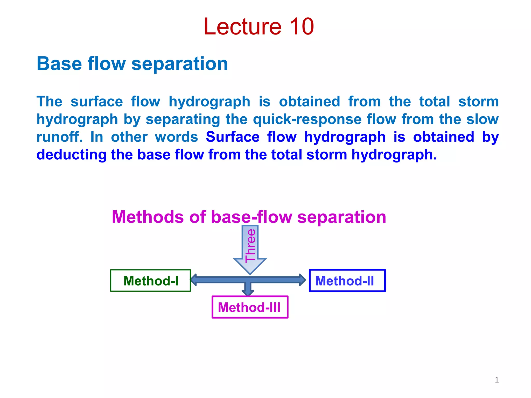
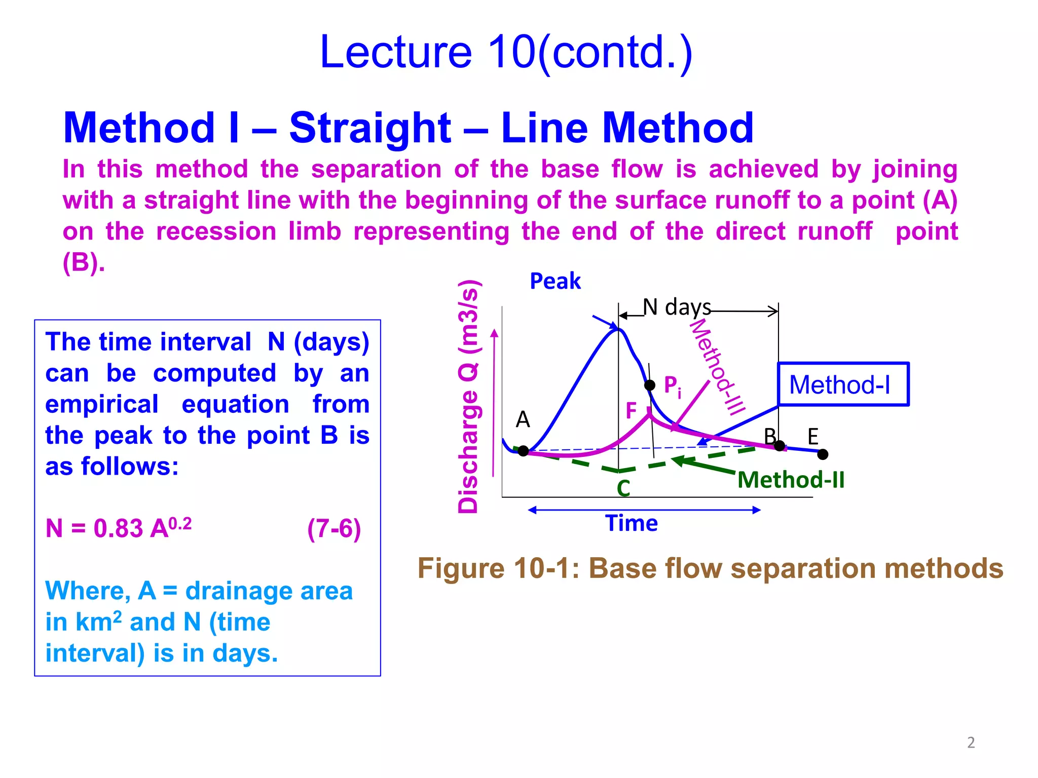
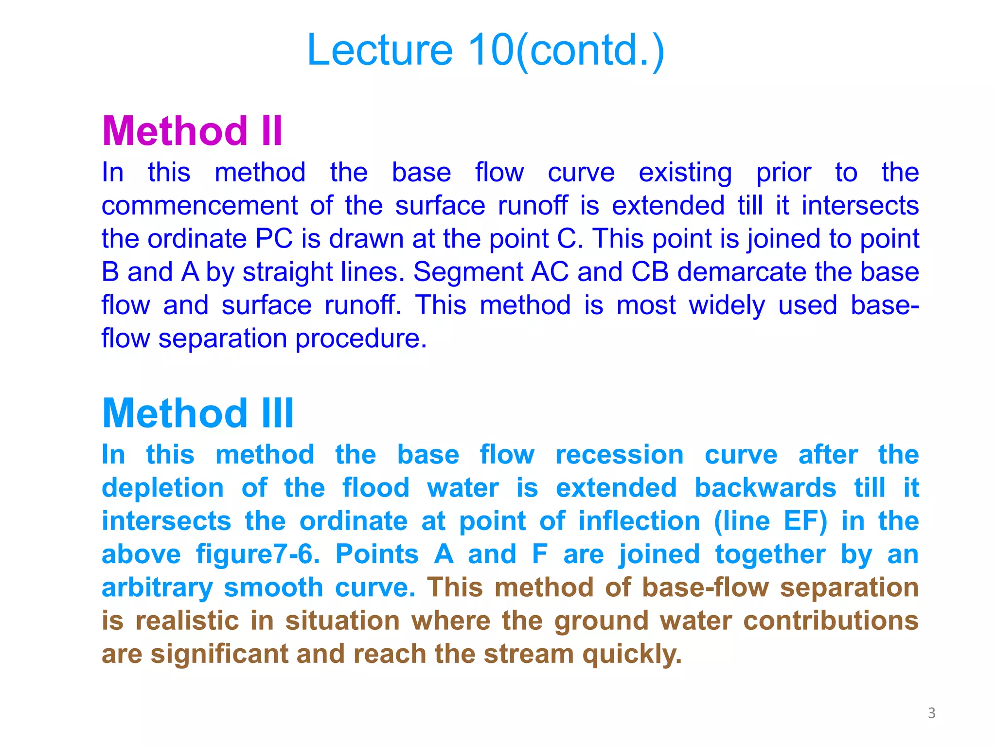
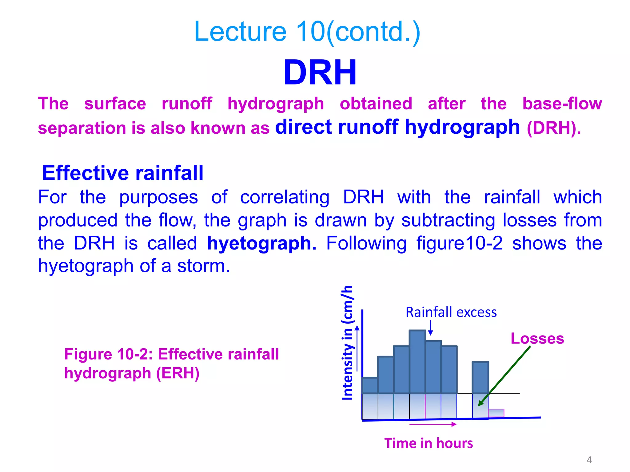
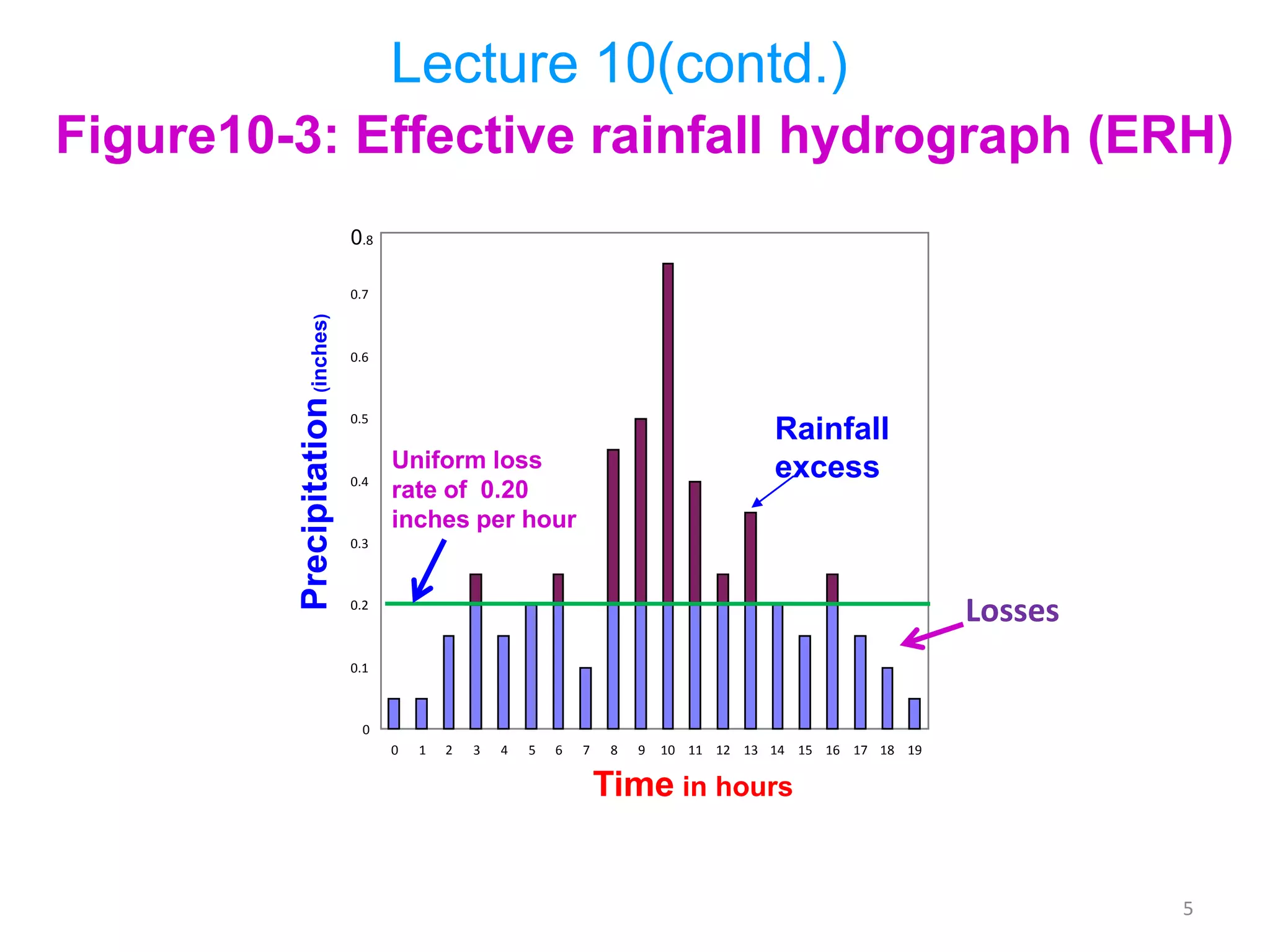
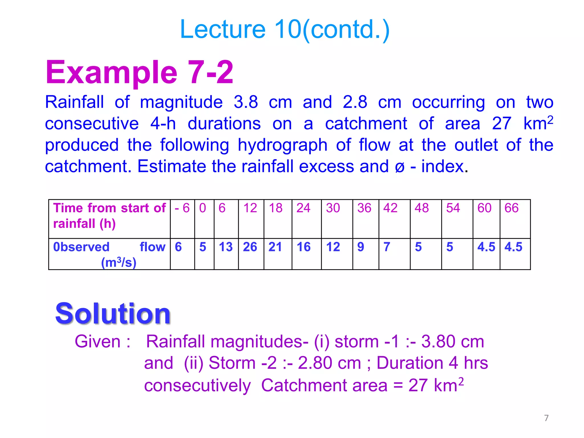
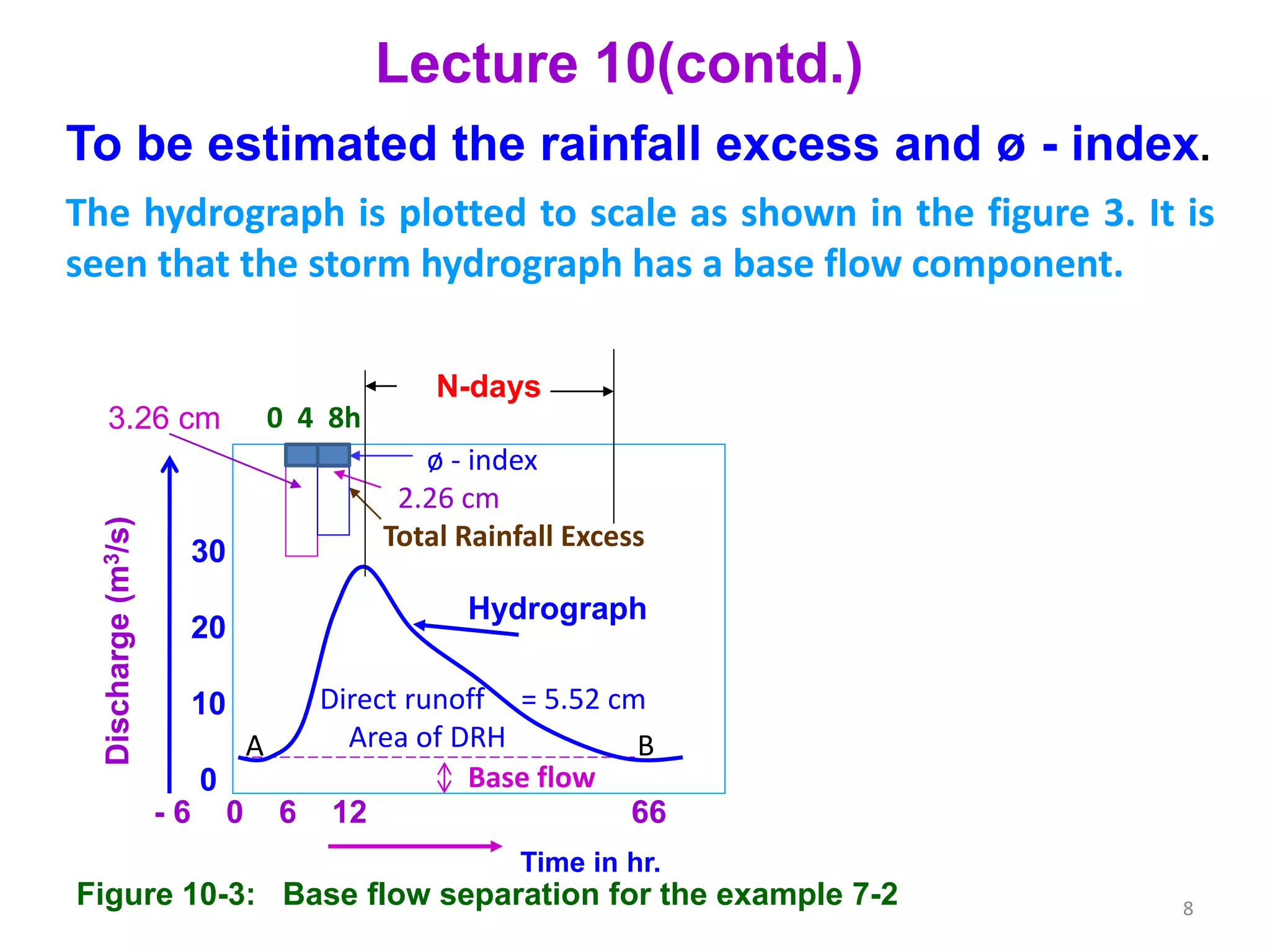
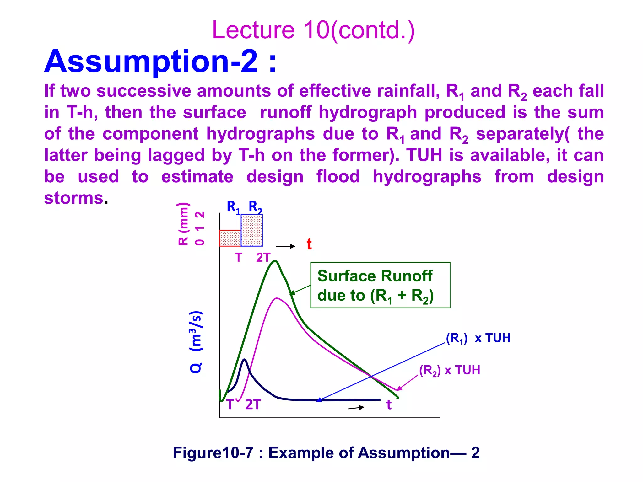
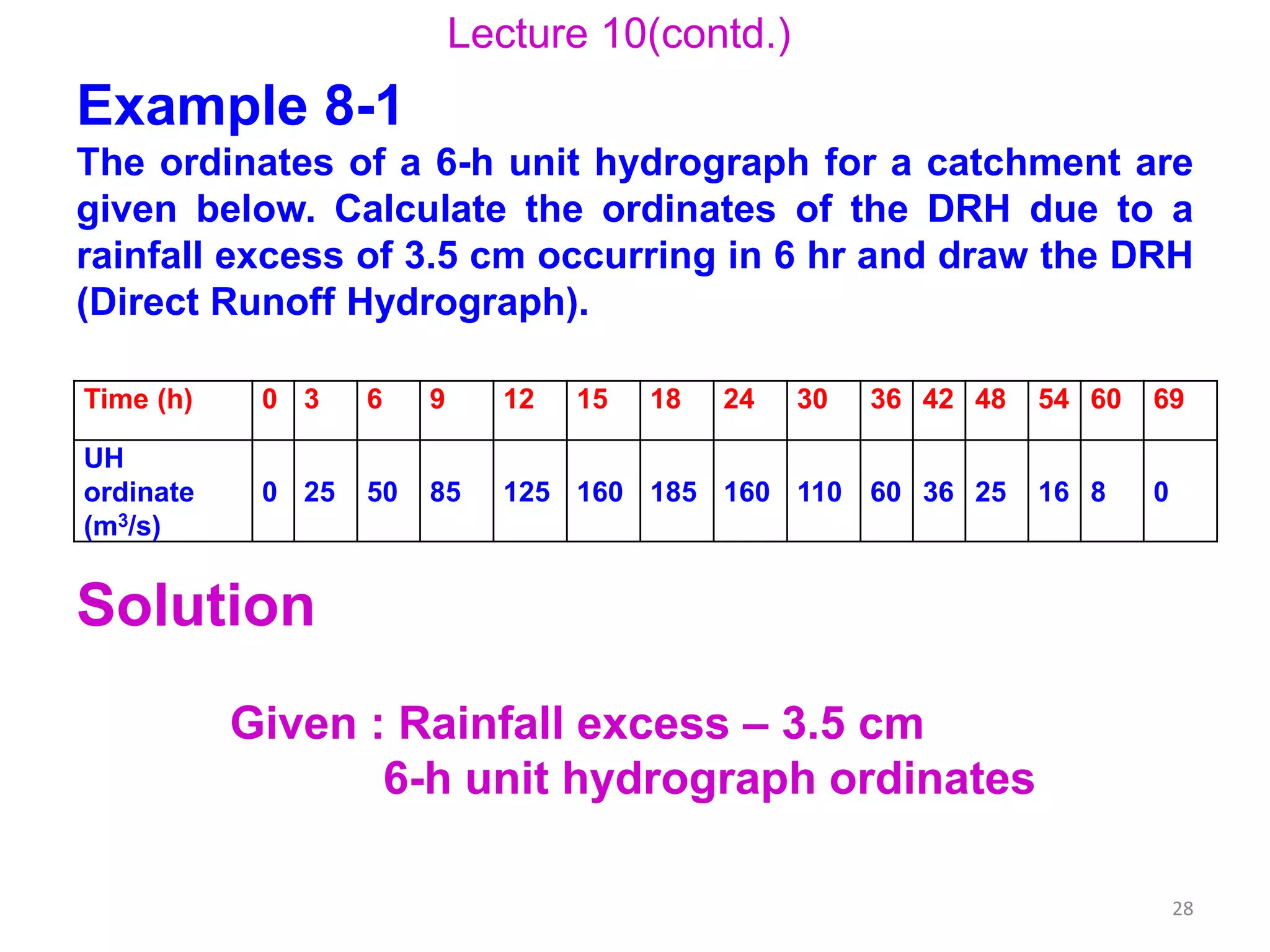
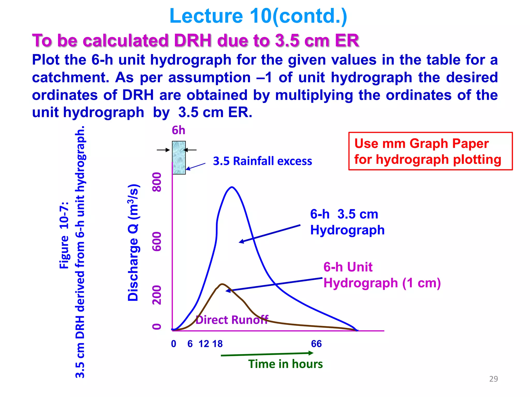
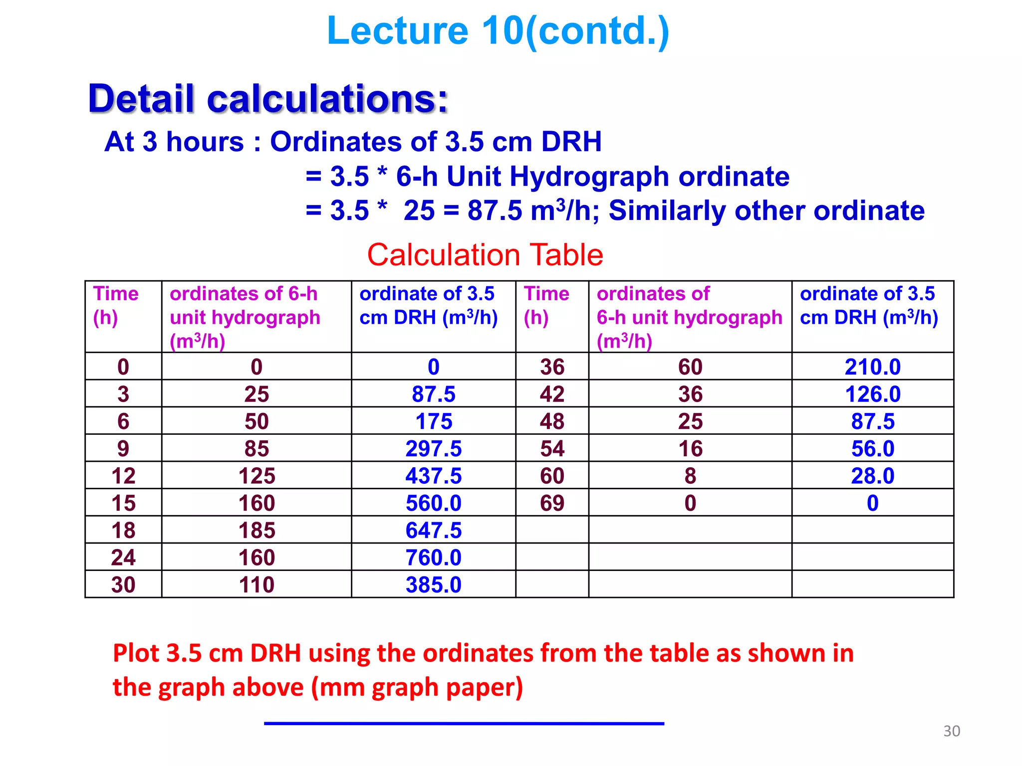
1
Lecture 10
Base flow separation
The surface flow hydrograph is obtained from the total storm
hydrograph by separating the quick-response flow from the slow
runoff. In other words Surface flow hydrograph is obtained by
deducting the base flow from the total storm hydrograph.
Methods of base-flow separation
Three
Method-IIMethod-I
Method-III
Lecture 10(contd.)
2
Figure 10-1: Base flow separation methods
DischargeQ(m3/s)
Time
Peak
N days
A
● ● ●
B E
Method-I● Pi
C
F
Method-II
Method I – Straight – Line Method
In this method the separation of the base flow is achieved by joining
with a straight line with the beginning of the surface runoff to a point (A)
on the recession limb representing the end of the direct runoff point
(B).
The time interval N (days)
can be computed by an
empirical equation from
the peak to the point B is
as follows:
N = 0.83 A0.2 (7-6)
Where, A = drainage area
in km2 and N (time
interval) is in days.
3
Lecture 10(contd.)
Method II
In this method the base flow curve existing prior to the
commencement of the surface runoff is extended till it intersects
the ordinate PC is drawn at the point C. This point is joined to point
B and A by straight lines. Segment AC and CB demarcate the base
flow and surface runoff. This method is most widely used base-
flow separation procedure.
Method III
In this method the base flow recession curve after the
depletion of the flood water is extended backwards till it
intersects the ordinate at point of inflection (line EF) in the
above figure7-6. Points A and F are joined together by an
arbitrary smooth curve. This method of base-flow separation
is realistic in situation where the ground water contributions
are significant and reach the stream quickly.
4
Lecture 10(contd.)
DRH
The surface runoff hydrograph obtained after the base-flow
separation is also known as direct runoff hydrograph (DRH).
Effective rainfall
For the purposes of correlating DRH with the rainfall which
produced the flow, the graph is drawn by subtracting losses from
the DRH is called hyetograph. Following figure10-2 shows the
hyetograph of a storm.
Rainfall excess
Losses
Time in hours
Intensityin(cm/hFigure 10-2: Effective rainfall
hydrograph (ERH)
5
0
0.1
0.2
0.3
0.4
0.5
0.6
0.7
0.8
0 1 2 3 4 5 6 7 8 9 10 11 12 13 14 15 16 17 18 19
Time in hours
Precipitation(inches)
Uniform loss
rate of 0.20
inches per hour
Lecture 10(contd.)
Losses
Rainfall
excess
Figure10-3: Effective rainfall hydrograph (ERH)
6
ERH
The hyetograph is drawn by subtracting initial losses and
infiltration losses from DRH is known as Effective Rainfall
Hyetograph(ERH) . It is also known as hyetograph of rainfall
excess or supra rainfall.
Both DRH and ERH represent the same total quantity but in
different units. Since ERH is usually in cm/h plotted against time,
Hence,
the total volume of direct runoff
= the area of ERH multiplied x the catchment area
This calculated volume is equal to the area of DRH.
Lecture 10(contd.)
7
Lecture 10(contd.)
Example 7-2
Rainfall of magnitude 3.8 cm and 2.8 cm occurring on two
consecutive 4-h durations on a catchment of area 27 km2
produced the following hydrograph of flow at the outlet of the
catchment. Estimate the rainfall excess and ø - index.
Time from start of
rainfall (h)
- 6 0 6 12 18 24 30 36 42 48 54 60 66
0bserved flow
(m3/s)
6 5 13 26 21 16 12 9 7 5 5 4.5 4.5
Solution
Given : Rainfall magnitudes- (i) storm -1 :- 3.80 cm
and (ii) Storm -2 :- 2.80 cm ; Duration 4 hrs
consecutively Catchment area = 27 km2
8
Lecture 10(contd.)
To be estimated the rainfall excess and ø - index.
The hydrograph is plotted to scale as shown in the figure 3. It is
seen that the storm hydrograph has a base flow component.
- 6 0 6 12 66
Discharge(m3/s)
30
20
10
0
0 4 8h3.26 cm
ø - index
2.26 cm
Total Rainfall Excess
Direct runoff = 5.52 cm
Area of DRH
Base flow
Time in hr.
Figure 10-3: Base flow separation for the example 7-2
Hydrograph
N-days
A B
9
Lecture 10(contd.)
First Base flow is separated by using Method-1 i.e. simple straight
line method of base flow separation.
Calculation of time from peak to end of depletion curve
N = 0.83 A0.2 ; A = 27 km2
or, N = 0.83 x270.2 = 1.6 days x24h =38.4, say, 38.5 h
However, From the figure, DRH starts at t = 0, and the peak at t= 12 h
and ends at t = 48 h. Hence the value of
N = 48 – 12 = 36 h which is more satisfactory than 38.5h,in this case.
DRH is assumed to exist from t = 0 to 48 h. A straight line base flow
separation gives a constant value of 5 m3/s for the base flow.
Lecture 10(contd.)
Base is equal to each segment, i.e. 12-6= 6 days and so on. Segment
area is almost triangular.
Hence, Area of DRH = 6 x 6ox60 { ½ (8) + ½ ( 8+21) + ½ (21+16) +
½ (16+ 11) + ½ ( 11+ 7) + ½ ( 7 + 4) + ½ (4+ 2) ½ ( 2)}
Area of DRH = 6 x 60x60 x ( 8 + 21+16+11+7+4+2) = 1.4904 x10⁶m3
Area of DRH = total direct runoff due to storm = 1.4904 x10⁶m3
Runoff depth = runoff volume / catchment area
Runoff depth = (1.4904 m3 x 106)/ (27 x 106) = 0.0552 m = 5.52 cm
Runoff depth = Direct runoff = 5.52 cm
11
Lecture 10(contd.)
Total rainfall = 3.8 + 2.8 = 6.6 cm
Duration = given consecutive 4-h i.e. = 4 + 4 = 8 h
ø - index. = (6.6 – 5.52)/8 = 0.135 cm/h
losses in 4 h = (ø – index) × t = 0.135 X 4 = 0.54 cm
Rainfall excess for first 4 h = (Total rainfall - losses)
= 3.80 – 0.54 = 3.26 cm
and next 4h = 2.8-0.54 = 2.26 cm
Ans ø - index = 0.135 cm /h and
rainfall excess: 3.26 and 2.26 cm
12
Lecture 10(contd.)
Example 7-3
A storm over a catchment of area 5.0 km2 had a duration of
14 hours rainfall. The data of mass curve of rainfall of the
storm is mentioned in the Data Table-1 below.
If the ө-index for the catchment is 0.4 cm/h, determine
the effective rainfall hyetograph and the volume of
direct runoff from the catchment due to the storm.
Time from start storm(h) 0 2 4 6 8 10 12 14
Accumulated rainfall(cm) 0 0.6 2.8 5.2 6.7 7.5 9.2 9.6
Solution
Given: Total rainfall duration = 14 hours;
Catchment area = 5.0 km2
ө-index for the catchment is 0.4 cm/h
13
Lecture 10(contd.)
To be calculated
(a)the effective rainfall hyetograph and the intensity of ER
(b) the volume of direct runoff from the catchment due to the storm.
(a) Calculation of effective rainfall hyetograph:
Time of rainfall interval, ∆t = (4-2) hr = (2-0) hr = 2 hr .
ө -index = 0.4 cm/h (given)
From the Data table: Actual depth of rainfall = 2.8 – 0.6 = 2.2 cm
ER = Effective Rainfall = Actual depth of rainfall – infiltration
ER = (From table )Actual depth of rainfall – ө ∆t = 2.2 – 0.4 × 2
= 1.4 cm and so on
ER = (actual depth of rainfall - ø ∆t) will be + ve
If , ER = - ve , then, ER = 0
14
Time from
start of
storm (h)
Time
interval
∆ t (h)
Accumulate
d rainfall in
∆t(cm)
Depth of
rainfall in ∆t
(cm)
ө ∆t
(cm)
ER
(cm)
Intensity of
ER (cm/h)
0 0 0 - - - -
2 2 0.6 0.6 0.8 0.0 0.0
4 2 2.8 2.2 0.8 1.4 0.7
6 2 5.2 2.4 0.8 1.6 0.8
8 2 6.7 1.5 0.8 0.7 0.35
10 2 7.5 0.8 0.8 0 0
12 2 9.2 1.7 0.8 0.9 0.45
14 2 9.6 0.4 0.8 0 0
Calculation Table
Total ER (effective rainfall) = Direct runoff due to storm
= Area of ER hyetograph
(a) Total ER = (0 + 0.7 + 0.8+0.35+0+ 0.45 + 0) ×2 = 4.60 cm
(b) Volume of Direct runoff = (4.6 / 100 ) x 5 km2
= (0.046 x 5 x (1000)2 = 230,000 m3
Lecture 10(contd.)
15
Lecture 10(contd.)
Rainfallintensity(cm/h)
0 2 4 6 8 10 12 14 16
Time in hours
0.7
0.8
0.35
0.45
0.1.2.3.4.5.6.7.8.91.0
Figure10-4: ERH of Storm for Example 7 -3
16
The hydrograph that results from unit depth (1-inch) of excess
precipitation (or runoff) spread uniformly in space and time over a
catchment for a given duration (D-hour) is called unit hydrograph.
The main points :
1-inch of EXCESS precipitation
Spread uniformly over space - evenly over the catchment
Uniformly in time - the excess rate is constant over the time
interval
There is a given duration
CHAPTER-8
UNIT HYDROGRAPH
Lecture 10(contd.)
17
Lecture 10(contd.)
USE OF UNIT HYDROGRAPH
The analysis of hydrological data found from storm to
storm in a known catchment, many problems arise to
predict the flood hydrograph. To solve this problem, there
are many methods. The unit hydrograph method is the
most popular and widely used. The unit hydrograph
method was first introduced by American engineer
Sherman in 1932.
18
Unit Hydrograph Theory
Sherman - 1932
Horton - 1933
Wisler & Brater - 1949 - “the hydrograph of surface runoff
resulting from a relatively short, intense rain, called a unit storm.”
Black, 1990 –
The runoff hydrograph may be “made up” of runoff that is
generated as flow through the soil
Lecture 10(contd.)
19
Unit Hydrograph Theory
Lecture 10(contd.)
20
Unit Hydrograph components
1. Duration
2. Lag Time
3. Time of Concentration
4. Rising Limb
5. Recession Limb (falling limb)
6. Peak Flow
7. Time to Peak (rise time)
8. Recession Curve
9. Separation
10. Base flow
Lecture 10(contd.)
21
Graphical Representation
Lag time
Time of concentration
Duration of excess
precipitation.
Base flow
Time
Discharge
Unit
hydrograph
Figure10-5
Peak
Lecture 10(contd.)
22
Lecture 10(contd.)
What does mean 2-hours Unit hydrograph?
It means unit hydrograph of 2 hours duration rainfall.
Generally it expresses as D-hours Unit hydrograph.
For the application of the unit hydrograph method
several assumptions has been considered: Some of
them are –
23
Q(m3/s)
R(mm)
012
T
0 T
Time
2 x TUH
Unit Hydrograph (TUH)
Lecture 10(contd.)
Figure10-6: Example of
Assumption—1
Assumption No.1 :
There is a direct proportional
relationship between the
effective rainfall and the surface
runoff. The figure-1 shows two
units of effective rainfall falling
in time T produce a surface
runoff hydrograph that has its
ordinates twice the TUH
ordinates, similarly for any
proportional value. For example,
if a 6.5 mm of effective rainfall
fall on a catchment area in T-h
then the hydrograph from that
effective rainfall will be by
multiplying the ordinates of the
TUH with the 6.5.
Lecture 10(contd.)
Assumption-2 :
If two successive amounts of effective rainfall, R1 and R2 each fall
in T-h, then the surface runoff hydrograph produced is the sum
of the component hydrographs due to R1 and R2 separately( the
latter being lagged by T-h on the former). TUH is available, it can
be used to estimate design flood hydrographs from design
storms. R1 R2
T 2T
t
R(mm)
012Q(m3/s)
T 2T t
Surface Runoff
due to (R1 + R2)
(R2) x TUH
(R1) x TUH
Figure10-7 : Example of Assumption— 2
25
Lecture 10(contd.)
Assumption -3:
The effective rainfall-surface runoff relationship does
not change with time, i.e. that the same TUH always
occurs whenever the unit of effective rainfall in T-h is
applied. Using this assumption of invariance, once a
TUH has been derived for a catchment area it could be
used to represent the response of the catchment
whenever required.
26
Weakness of unit hydrograph method
1. The assumptions of unit hydrograph must be applied to natural
Catchment
2. In relating, effective rainfall to surface runoff, the amount of
effective rainfall depends on the state of the catchment before
the storm event.
3. Only when the ground deficiencies have been made up and the
rainfall becomes fully effective will extra rainfall in the same
time period produce proportionally more runoff.
4. The first assumption of proportionality of response to the
effective rainfall conflicts with the observed non-proportional
behavior of river flow.
5. In a second period of effective rain, the response of a catchment
will be dependent on the effects of the first input.
Lecture 10(contd.)
27
6. The third assumption of time invariance implies
that whatever the state of the catchment, a unit
of effective rainfall in T-h will always produce
the same TUH. But the response of hydrograph
of a catchment must vary according to the
season.
7. Another weakness of the unit hydrograph
method is the assumption that the effective
rainfall is produced uniformly both in the time T
and over the area of the catchment.
Lecture 10(contd.)
Weakness of unit hydrograph method
(contd.)
28
Lecture 10(contd.)
Example 8-1
The ordinates of a 6-h unit hydrograph for a catchment are
given below. Calculate the ordinates of the DRH due to a
rainfall excess of 3.5 cm occurring in 6 hr and draw the DRH
(Direct Runoff Hydrograph).
Time (h) 0 3 6 9 12 15 18 24 30 36 42 48 54 60 69
UH
ordinate
(m3/s)
0 25 50 85 125 160 185 160 110 60 36 25 16 8 0
Solution
Given : Rainfall excess – 3.5 cm
6-h unit hydrograph ordinates
29
6h
3.5 Rainfall excess
6-h Unit
Hydrograph (1 cm)
0 6 12 18 66
0200600800
DischargeQ(m3/s)
Direct Runoff
Time in hours
6-h 3.5 cm
Hydrograph
Figure10-7:
3.5cmDRHderivedfrom6-hunithydrograph.
To be calculated DRH due to 3.5 cm ER
Plot the 6-h unit hydrograph for the given values in the table for a
catchment. As per assumption –1 of unit hydrograph the desired
ordinates of DRH are obtained by multiplying the ordinates of the
unit hydrograph by 3.5 cm ER.
Lecture 10(contd.)
Use mm Graph Paper
for hydrograph plotting
30
Time
(h)
ordinates of 6-h
unit hydrograph
(m3/h)
ordinate of 3.5
cm DRH (m3/h)
Time
(h)
ordinates of
6-h unit hydrograph
(m3/h)
ordinate of 3.5
cm DRH (m3/h)
0 0 0 36 60 210.0
3 25 87.5 42 36 126.0
6 50 175 48 25 87.5
9 85 297.5 54 16 56.0
12 125 437.5 60 8 28.0
15 160 560.0 69 0 0
18 185 647.5
24 160 760.0
30 110 385.0
Calculation Table
Detail calculations:
At 3 hours : Ordinates of 3.5 cm DRH
= 3.5 * 6-h Unit Hydrograph ordinate
= 3.5 * 25 = 87.5 m3/h; Similarly other ordinate
Plot 3.5 cm DRH using the ordinates from the table as shown in
the graph above (mm graph paper)
Lecture 10(contd.)

Class lecture on Hydrology by Rabindra Ranjan saha Lecture 10

  • 1.
    1 Lecture 10 Base flowseparation The surface flow hydrograph is obtained from the total storm hydrograph by separating the quick-response flow from the slow runoff. In other words Surface flow hydrograph is obtained by deducting the base flow from the total storm hydrograph. Methods of base-flow separation Three Method-IIMethod-I Method-III
  • 2.
    Lecture 10(contd.) 2 Figure 10-1:Base flow separation methods DischargeQ(m3/s) Time Peak N days A ● ● ● B E Method-I● Pi C F Method-II Method I – Straight – Line Method In this method the separation of the base flow is achieved by joining with a straight line with the beginning of the surface runoff to a point (A) on the recession limb representing the end of the direct runoff point (B). The time interval N (days) can be computed by an empirical equation from the peak to the point B is as follows: N = 0.83 A0.2 (7-6) Where, A = drainage area in km2 and N (time interval) is in days.
  • 3.
    3 Lecture 10(contd.) Method II Inthis method the base flow curve existing prior to the commencement of the surface runoff is extended till it intersects the ordinate PC is drawn at the point C. This point is joined to point B and A by straight lines. Segment AC and CB demarcate the base flow and surface runoff. This method is most widely used base- flow separation procedure. Method III In this method the base flow recession curve after the depletion of the flood water is extended backwards till it intersects the ordinate at point of inflection (line EF) in the above figure7-6. Points A and F are joined together by an arbitrary smooth curve. This method of base-flow separation is realistic in situation where the ground water contributions are significant and reach the stream quickly.
  • 4.
    4 Lecture 10(contd.) DRH The surfacerunoff hydrograph obtained after the base-flow separation is also known as direct runoff hydrograph (DRH). Effective rainfall For the purposes of correlating DRH with the rainfall which produced the flow, the graph is drawn by subtracting losses from the DRH is called hyetograph. Following figure10-2 shows the hyetograph of a storm. Rainfall excess Losses Time in hours Intensityin(cm/hFigure 10-2: Effective rainfall hydrograph (ERH)
  • 5.
    5 0 0.1 0.2 0.3 0.4 0.5 0.6 0.7 0.8 0 1 23 4 5 6 7 8 9 10 11 12 13 14 15 16 17 18 19 Time in hours Precipitation(inches) Uniform loss rate of 0.20 inches per hour Lecture 10(contd.) Losses Rainfall excess Figure10-3: Effective rainfall hydrograph (ERH)
  • 6.
    6 ERH The hyetograph isdrawn by subtracting initial losses and infiltration losses from DRH is known as Effective Rainfall Hyetograph(ERH) . It is also known as hyetograph of rainfall excess or supra rainfall. Both DRH and ERH represent the same total quantity but in different units. Since ERH is usually in cm/h plotted against time, Hence, the total volume of direct runoff = the area of ERH multiplied x the catchment area This calculated volume is equal to the area of DRH. Lecture 10(contd.)
  • 7.
    7 Lecture 10(contd.) Example 7-2 Rainfallof magnitude 3.8 cm and 2.8 cm occurring on two consecutive 4-h durations on a catchment of area 27 km2 produced the following hydrograph of flow at the outlet of the catchment. Estimate the rainfall excess and ø - index. Time from start of rainfall (h) - 6 0 6 12 18 24 30 36 42 48 54 60 66 0bserved flow (m3/s) 6 5 13 26 21 16 12 9 7 5 5 4.5 4.5 Solution Given : Rainfall magnitudes- (i) storm -1 :- 3.80 cm and (ii) Storm -2 :- 2.80 cm ; Duration 4 hrs consecutively Catchment area = 27 km2
  • 8.
    8 Lecture 10(contd.) To beestimated the rainfall excess and ø - index. The hydrograph is plotted to scale as shown in the figure 3. It is seen that the storm hydrograph has a base flow component. - 6 0 6 12 66 Discharge(m3/s) 30 20 10 0 0 4 8h3.26 cm ø - index 2.26 cm Total Rainfall Excess Direct runoff = 5.52 cm Area of DRH Base flow Time in hr. Figure 10-3: Base flow separation for the example 7-2 Hydrograph N-days A B
  • 9.
    9 Lecture 10(contd.) First Baseflow is separated by using Method-1 i.e. simple straight line method of base flow separation. Calculation of time from peak to end of depletion curve N = 0.83 A0.2 ; A = 27 km2 or, N = 0.83 x270.2 = 1.6 days x24h =38.4, say, 38.5 h However, From the figure, DRH starts at t = 0, and the peak at t= 12 h and ends at t = 48 h. Hence the value of N = 48 – 12 = 36 h which is more satisfactory than 38.5h,in this case. DRH is assumed to exist from t = 0 to 48 h. A straight line base flow separation gives a constant value of 5 m3/s for the base flow.
  • 10.
    Lecture 10(contd.) Base isequal to each segment, i.e. 12-6= 6 days and so on. Segment area is almost triangular. Hence, Area of DRH = 6 x 6ox60 { ½ (8) + ½ ( 8+21) + ½ (21+16) + ½ (16+ 11) + ½ ( 11+ 7) + ½ ( 7 + 4) + ½ (4+ 2) ½ ( 2)} Area of DRH = 6 x 60x60 x ( 8 + 21+16+11+7+4+2) = 1.4904 x10⁶m3 Area of DRH = total direct runoff due to storm = 1.4904 x10⁶m3 Runoff depth = runoff volume / catchment area Runoff depth = (1.4904 m3 x 106)/ (27 x 106) = 0.0552 m = 5.52 cm Runoff depth = Direct runoff = 5.52 cm
  • 11.
    11 Lecture 10(contd.) Total rainfall= 3.8 + 2.8 = 6.6 cm Duration = given consecutive 4-h i.e. = 4 + 4 = 8 h ø - index. = (6.6 – 5.52)/8 = 0.135 cm/h losses in 4 h = (ø – index) × t = 0.135 X 4 = 0.54 cm Rainfall excess for first 4 h = (Total rainfall - losses) = 3.80 – 0.54 = 3.26 cm and next 4h = 2.8-0.54 = 2.26 cm Ans ø - index = 0.135 cm /h and rainfall excess: 3.26 and 2.26 cm
  • 12.
    12 Lecture 10(contd.) Example 7-3 Astorm over a catchment of area 5.0 km2 had a duration of 14 hours rainfall. The data of mass curve of rainfall of the storm is mentioned in the Data Table-1 below. If the ө-index for the catchment is 0.4 cm/h, determine the effective rainfall hyetograph and the volume of direct runoff from the catchment due to the storm. Time from start storm(h) 0 2 4 6 8 10 12 14 Accumulated rainfall(cm) 0 0.6 2.8 5.2 6.7 7.5 9.2 9.6 Solution Given: Total rainfall duration = 14 hours; Catchment area = 5.0 km2 ө-index for the catchment is 0.4 cm/h
  • 13.
    13 Lecture 10(contd.) To becalculated (a)the effective rainfall hyetograph and the intensity of ER (b) the volume of direct runoff from the catchment due to the storm. (a) Calculation of effective rainfall hyetograph: Time of rainfall interval, ∆t = (4-2) hr = (2-0) hr = 2 hr . ө -index = 0.4 cm/h (given) From the Data table: Actual depth of rainfall = 2.8 – 0.6 = 2.2 cm ER = Effective Rainfall = Actual depth of rainfall – infiltration ER = (From table )Actual depth of rainfall – ө ∆t = 2.2 – 0.4 × 2 = 1.4 cm and so on ER = (actual depth of rainfall - ø ∆t) will be + ve If , ER = - ve , then, ER = 0
  • 14.
    14 Time from start of storm(h) Time interval ∆ t (h) Accumulate d rainfall in ∆t(cm) Depth of rainfall in ∆t (cm) ө ∆t (cm) ER (cm) Intensity of ER (cm/h) 0 0 0 - - - - 2 2 0.6 0.6 0.8 0.0 0.0 4 2 2.8 2.2 0.8 1.4 0.7 6 2 5.2 2.4 0.8 1.6 0.8 8 2 6.7 1.5 0.8 0.7 0.35 10 2 7.5 0.8 0.8 0 0 12 2 9.2 1.7 0.8 0.9 0.45 14 2 9.6 0.4 0.8 0 0 Calculation Table Total ER (effective rainfall) = Direct runoff due to storm = Area of ER hyetograph (a) Total ER = (0 + 0.7 + 0.8+0.35+0+ 0.45 + 0) ×2 = 4.60 cm (b) Volume of Direct runoff = (4.6 / 100 ) x 5 km2 = (0.046 x 5 x (1000)2 = 230,000 m3 Lecture 10(contd.)
  • 15.
    15 Lecture 10(contd.) Rainfallintensity(cm/h) 0 24 6 8 10 12 14 16 Time in hours 0.7 0.8 0.35 0.45 0.1.2.3.4.5.6.7.8.91.0 Figure10-4: ERH of Storm for Example 7 -3
  • 16.
    16 The hydrograph thatresults from unit depth (1-inch) of excess precipitation (or runoff) spread uniformly in space and time over a catchment for a given duration (D-hour) is called unit hydrograph. The main points : 1-inch of EXCESS precipitation Spread uniformly over space - evenly over the catchment Uniformly in time - the excess rate is constant over the time interval There is a given duration CHAPTER-8 UNIT HYDROGRAPH Lecture 10(contd.)
  • 17.
    17 Lecture 10(contd.) USE OFUNIT HYDROGRAPH The analysis of hydrological data found from storm to storm in a known catchment, many problems arise to predict the flood hydrograph. To solve this problem, there are many methods. The unit hydrograph method is the most popular and widely used. The unit hydrograph method was first introduced by American engineer Sherman in 1932.
  • 18.
    18 Unit Hydrograph Theory Sherman- 1932 Horton - 1933 Wisler & Brater - 1949 - “the hydrograph of surface runoff resulting from a relatively short, intense rain, called a unit storm.” Black, 1990 – The runoff hydrograph may be “made up” of runoff that is generated as flow through the soil Lecture 10(contd.)
  • 19.
  • 20.
    20 Unit Hydrograph components 1.Duration 2. Lag Time 3. Time of Concentration 4. Rising Limb 5. Recession Limb (falling limb) 6. Peak Flow 7. Time to Peak (rise time) 8. Recession Curve 9. Separation 10. Base flow Lecture 10(contd.)
  • 21.
    21 Graphical Representation Lag time Timeof concentration Duration of excess precipitation. Base flow Time Discharge Unit hydrograph Figure10-5 Peak Lecture 10(contd.)
  • 22.
    22 Lecture 10(contd.) What doesmean 2-hours Unit hydrograph? It means unit hydrograph of 2 hours duration rainfall. Generally it expresses as D-hours Unit hydrograph. For the application of the unit hydrograph method several assumptions has been considered: Some of them are –
  • 23.
    23 Q(m3/s) R(mm) 012 T 0 T Time 2 xTUH Unit Hydrograph (TUH) Lecture 10(contd.) Figure10-6: Example of Assumption—1 Assumption No.1 : There is a direct proportional relationship between the effective rainfall and the surface runoff. The figure-1 shows two units of effective rainfall falling in time T produce a surface runoff hydrograph that has its ordinates twice the TUH ordinates, similarly for any proportional value. For example, if a 6.5 mm of effective rainfall fall on a catchment area in T-h then the hydrograph from that effective rainfall will be by multiplying the ordinates of the TUH with the 6.5.
  • 24.
    Lecture 10(contd.) Assumption-2 : Iftwo successive amounts of effective rainfall, R1 and R2 each fall in T-h, then the surface runoff hydrograph produced is the sum of the component hydrographs due to R1 and R2 separately( the latter being lagged by T-h on the former). TUH is available, it can be used to estimate design flood hydrographs from design storms. R1 R2 T 2T t R(mm) 012Q(m3/s) T 2T t Surface Runoff due to (R1 + R2) (R2) x TUH (R1) x TUH Figure10-7 : Example of Assumption— 2
  • 25.
    25 Lecture 10(contd.) Assumption -3: Theeffective rainfall-surface runoff relationship does not change with time, i.e. that the same TUH always occurs whenever the unit of effective rainfall in T-h is applied. Using this assumption of invariance, once a TUH has been derived for a catchment area it could be used to represent the response of the catchment whenever required.
  • 26.
    26 Weakness of unithydrograph method 1. The assumptions of unit hydrograph must be applied to natural Catchment 2. In relating, effective rainfall to surface runoff, the amount of effective rainfall depends on the state of the catchment before the storm event. 3. Only when the ground deficiencies have been made up and the rainfall becomes fully effective will extra rainfall in the same time period produce proportionally more runoff. 4. The first assumption of proportionality of response to the effective rainfall conflicts with the observed non-proportional behavior of river flow. 5. In a second period of effective rain, the response of a catchment will be dependent on the effects of the first input. Lecture 10(contd.)
  • 27.
    27 6. The thirdassumption of time invariance implies that whatever the state of the catchment, a unit of effective rainfall in T-h will always produce the same TUH. But the response of hydrograph of a catchment must vary according to the season. 7. Another weakness of the unit hydrograph method is the assumption that the effective rainfall is produced uniformly both in the time T and over the area of the catchment. Lecture 10(contd.) Weakness of unit hydrograph method (contd.)
  • 28.
    28 Lecture 10(contd.) Example 8-1 Theordinates of a 6-h unit hydrograph for a catchment are given below. Calculate the ordinates of the DRH due to a rainfall excess of 3.5 cm occurring in 6 hr and draw the DRH (Direct Runoff Hydrograph). Time (h) 0 3 6 9 12 15 18 24 30 36 42 48 54 60 69 UH ordinate (m3/s) 0 25 50 85 125 160 185 160 110 60 36 25 16 8 0 Solution Given : Rainfall excess – 3.5 cm 6-h unit hydrograph ordinates
  • 29.
    29 6h 3.5 Rainfall excess 6-hUnit Hydrograph (1 cm) 0 6 12 18 66 0200600800 DischargeQ(m3/s) Direct Runoff Time in hours 6-h 3.5 cm Hydrograph Figure10-7: 3.5cmDRHderivedfrom6-hunithydrograph. To be calculated DRH due to 3.5 cm ER Plot the 6-h unit hydrograph for the given values in the table for a catchment. As per assumption –1 of unit hydrograph the desired ordinates of DRH are obtained by multiplying the ordinates of the unit hydrograph by 3.5 cm ER. Lecture 10(contd.) Use mm Graph Paper for hydrograph plotting
  • 30.
    30 Time (h) ordinates of 6-h unithydrograph (m3/h) ordinate of 3.5 cm DRH (m3/h) Time (h) ordinates of 6-h unit hydrograph (m3/h) ordinate of 3.5 cm DRH (m3/h) 0 0 0 36 60 210.0 3 25 87.5 42 36 126.0 6 50 175 48 25 87.5 9 85 297.5 54 16 56.0 12 125 437.5 60 8 28.0 15 160 560.0 69 0 0 18 185 647.5 24 160 760.0 30 110 385.0 Calculation Table Detail calculations: At 3 hours : Ordinates of 3.5 cm DRH = 3.5 * 6-h Unit Hydrograph ordinate = 3.5 * 25 = 87.5 m3/h; Similarly other ordinate Plot 3.5 cm DRH using the ordinates from the table as shown in the graph above (mm graph paper) Lecture 10(contd.)