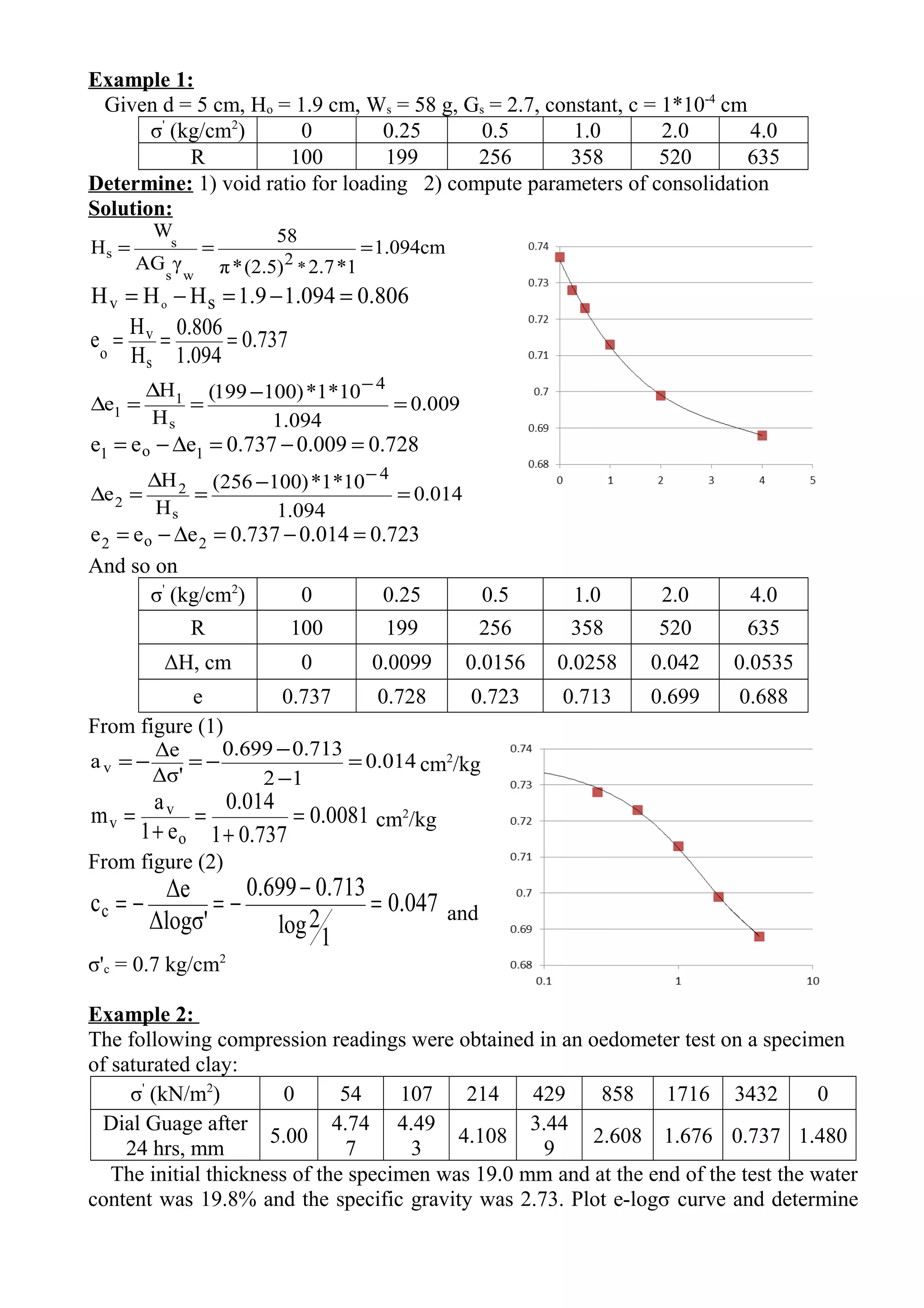
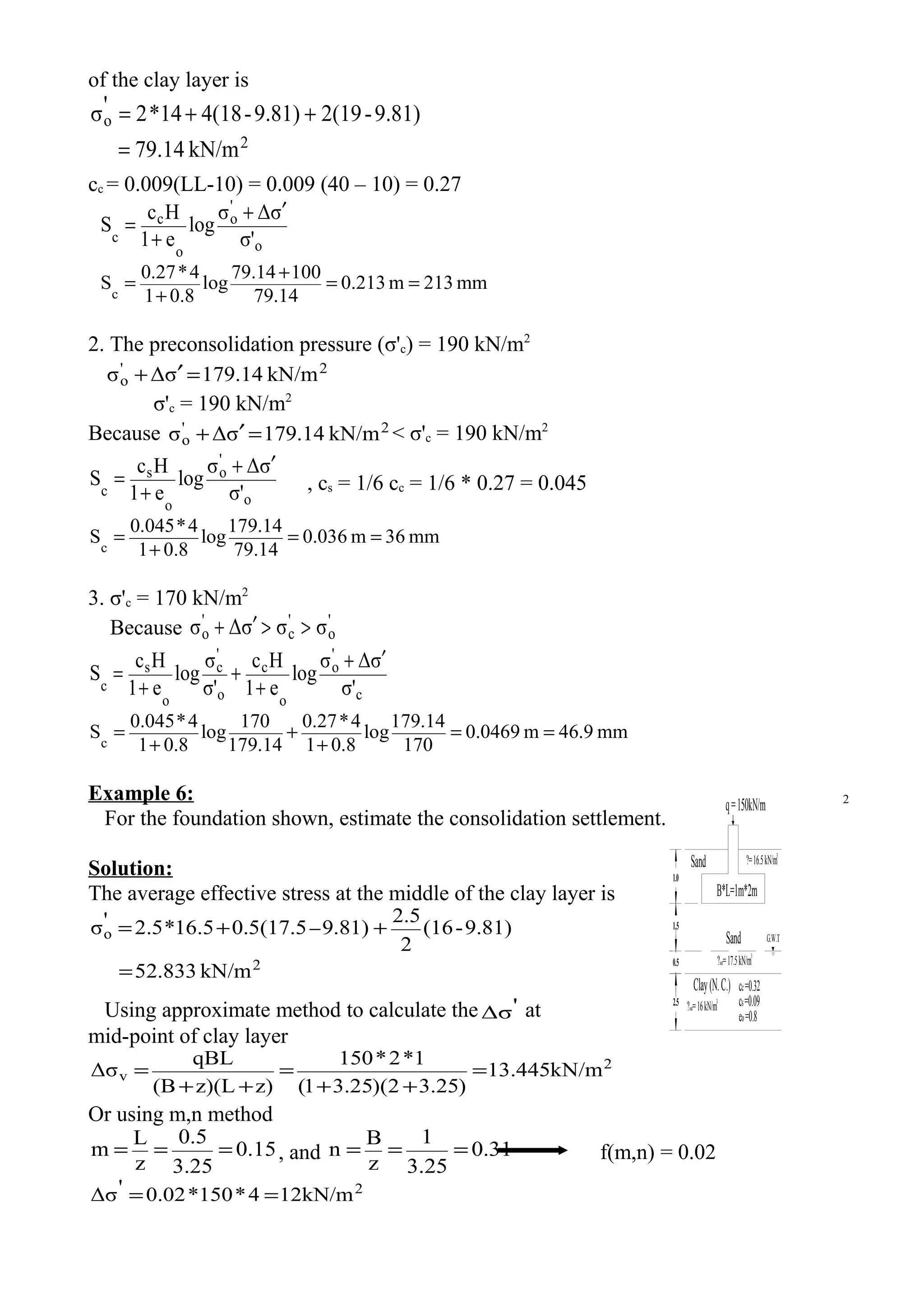
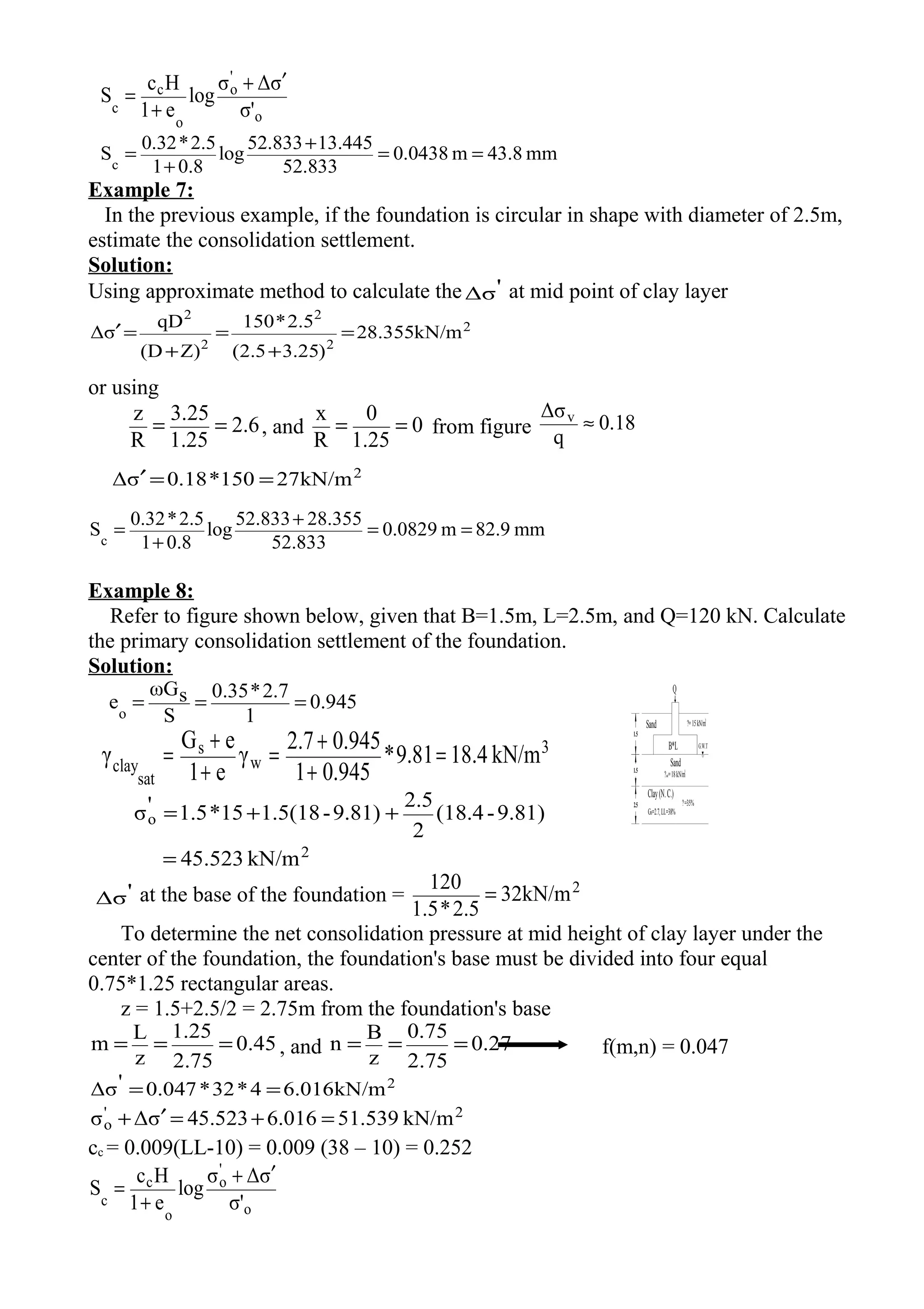
1. The document provides examples of calculating consolidation parameters such as void ratio, coefficient of consolidation, and primary consolidation settlement from given soil testing data. 2. Parameters like initial void ratio, applied pressure, and thickness of soil layers are used to determine the change in stress and void ratio to then calculate settlement. 3. Several methods are presented to calculate the average effective stress and stress change at different points to then determine the consolidation settlement under different boundary conditions, stress histories, and soil properties.

1. Example 1:
Given d = 5 cm, Ho = 1.9 cm, Ws = 58 g, Gs = 2.7, constant, c = 1*10-4
cm
σ'
(kg/cm2
) 0 0.25 0.5 1.0 2.0 4.0
R 100 199 256 358 520 635
Determine: 1) void ratio for loading 2) compute parameters of consolidation
Solution:
cm094.1
1*2.7(2.5)*π
58
γAG
W
H
*
2
ws
s
s ===
806.0094.19.1HHH sov =−=−=
737.0
1.094
0.806
H
H
e
s
v
o
===
009.0
094.1
10*1*)100199(
H
H
e
4
s
1
1 =
−
=
∆
=∆
−
728.0009.0737.0eee 1o1 =−=∆−=
014.0
094.1
10*1*)100256(
H
H
e
4
s
2
2 =
−
=
∆
=∆
−
723.0014.0737.0eee 2o2 =−=∆−=
And so on
σ'
(kg/cm2
) 0 0.25 0.5 1.0 2.0 4.0
R 100 199 256 358 520 635
ΔH, cm 0 0.0099 0.0156 0.0258 0.042 0.0535
e 0.737 0.728 0.723 0.713 0.699 0.688
From figure (1)
014.0
12
713.0699.0
Δσ'
Δe
av =
−
−
−=−= cm2
/kg
0081.0
737.01
014.0
e1
a
m
o
v
v =
+
=
+
= cm2
/kg
From figure (2)
047.0
1
2log
713.0699.0
Δlogσ'
Δe
cc =
−
−=−= and
σ'c = 0.7 kg/cm2
Example 2:
The following compression readings were obtained in an oedometer test on a specimen
of saturated clay:
σ'
(kN/m2
) 0 54 107 214 429 858 1716 3432 0
Dial Guage after
24 hrs, mm
5.00
4.74
7
4.49
3
4.108
3.44
9
2.608 1.676 0.737 1.480
The initial thickness of the specimen was 19.0 mm and at the end of the test the water
content was 19.8% and the specific gravity was 2.73. Plot e-logσ curve and determine

2. the coefficient of compressibility between 100-200 and 1000-1500 kN/m2
. What is the
value of cc for the latter increment?
Solution:
Void ratio at the end of the test = ef = ωGs= 0.198*2.73 = 0.541
Void ratio at the start of the test = eo = ef + ∆e
Now,
ee1
e
e1
e
H
H
foo
∆++
∆
=
+
∆
=
∆
350.0e
e0.5411
e
0.19
48.15
=∆⇒
∆++
∆
=
−
eo = ef + ∆e = 0.541 + 0.35 = 0.891
In general the relationship between ∆e and ∆H is given by:
891.01
e
19.0
H
e1
e
H
H
oo
+
∆
=
∆
⇒
+
∆
=
∆
H0995.0e ∆=∆⇒ , and can be used to obtain the void ratio at the end of each
increment period.
σ'
(kN/m2
) 0 54 107 214 429 858 1716 3432 0
Dial Guage
after 24 hrs,
mm
5.00
4.74
7
4.49
3
4.108
3.44
9
2.608 1.676 0.737 1.480
∆H, mm 0
0.25
3
0.50
7
0.892
1.55
1
2.392 3.324 4.263 3.520
∆e 0
0.02
5
0.05
0
0.089
0.15
4
0.238 0.331 0.424 0.350
e
0.89
1
0.86
6
0.84
1
0.802
0.73
7
0.653 0.560 0.467 0.541
e1 = eo – ∆e = 0.891 – 0.025 =0.866
0.891 – 0.05 = 0.841
The e-logσ curve using these values is shown in figure below. Using Casagrande’s
construction the value of the preconsolidation pressure is 325 kN/m3
.
Between the pressure range
100 and 200 kN/m2
e100= 0.845 e200= 0.808, therefore
/kNm10*7.3
100200
808.0845.0
Δσ'
Δe
a 24
v
−
=
−
−
−=−=
/kNm10*005.2
845.01
10*7.3
e1
a
m 24
4
v
v
−
−
=
+
=
+
=
Between the pressure range
1000 and 1500 kN/m2
e1000= 0.632 e1500= 0.577, therefore
/kNm10*1.1
10001500
577.0632.0
Δσ'
Δe
a 24
v
−
=
−
−
−=−=

3. /kNm10*74.6
632.01
10*1.1
e1
a
m 25
4
v
v
−
−
=
+
=
+
=
and
312.0
100
1500log
577.0632.0
Δlogσ'
Δe
cc =
−
−=−=
Example 3:
Compute the expected settlement of a building constructed on a soil layer of 2.5m
thick its e = 0.72, the pressure increased from 1.5 kg/cm2
to 3.8 kg/cm2
and caused
reduction in void ratio by 15%.
Solution:
e1 = 0.72(1 – 0.15) = 0.612
method 1
cm15.7m157.05.2*
72.01
0.6120.72
H.
e1
Δe
S
o
c
==
+
−
=
+
=
method 2
047.0
5.18.3
612.072.0
Δσ'
Δe
av =
−
−
==
027.0
72.01
047.0
e1
a
m
o
v
v =
+
=
+
=
cm15.5m0.1551.5)(3.8*2.5*0.027σHmS **vc
===′∆= −
Example 4:
For the system shown below, determine the primary consolidation settlement if cs =
0.05 for the following:
1) σ'c = 100 kPa 2) σ'c = 150 kPa 3) σ'c = 175 kPa 4) σ'c = 250 kPa
Solution:
1) σ'c = 100 kPa
σ'o at midpoint of the clay layer
2
o
kN/m150.85
9.7*19.81)5(19.718.7*5'σ
=
++= −
1663.0
85.150
100
σ
σ
OCR '
o
'
c
<=== therefore, under
]
'Δσσ'
σ
log
σ'
σΔσ
[log
e1
Hc
S
avo
'
o
o
'
o
o
c
c
−
+
′+
+
=
425.25)10085.150(
2
1
)σσ(
2
1'Δσ '
c
'
oav
=−== − kPa

4. 162mm0.162m]
25.425150.85
150.85
log
150.85
50150.85
[log
1.11
2*0.83
Sc
==+
+
+
=
−
2) σ'c = 150 kPa
1
85.150
150
σ
σ
OCR '
o
'
c
≈== normal
o
'
o
o
c
c σ'
σΔσ
log
e1
Hc
S
′+
+
=
mm98m098.0
150.85
50150.85
log
1.11
2*0.83
Sc
==
+
+
=
3) σ'c = 175 kPa
16.1
85.150
175
σ
σ
OCR '
o
'
c ===
kPa200.855085.150σΔσ'
o =+=′+
σ'c = 175 kPa
Because kPa200.85σΔσ'
o =′+ > σ'c = 175 kPa
c
'
o
o
c
o
'
c
o
s
c σ'
σΔσ
log
e1
Hc
σ'
σ
log
e1
Hc
S
′+
+
+
+
=
mm50.4m.05040
175
50150.85
log
1.11
2*0.83
150.85
175
log
1.11
2*0.05
Sc
==
+
+
+
+
=
4) σ'c = 250 kPa
Because kPa200.85σΔσ'
o =′+ < σ'c = 250 kPa
o
'
o
o
s
c σ'
σΔσ
log
e1
Hc
S
′+
+
=
mm6m0.006
150.85
50150.85
log
1.11
2*0.05
Sc
==
+
+
=
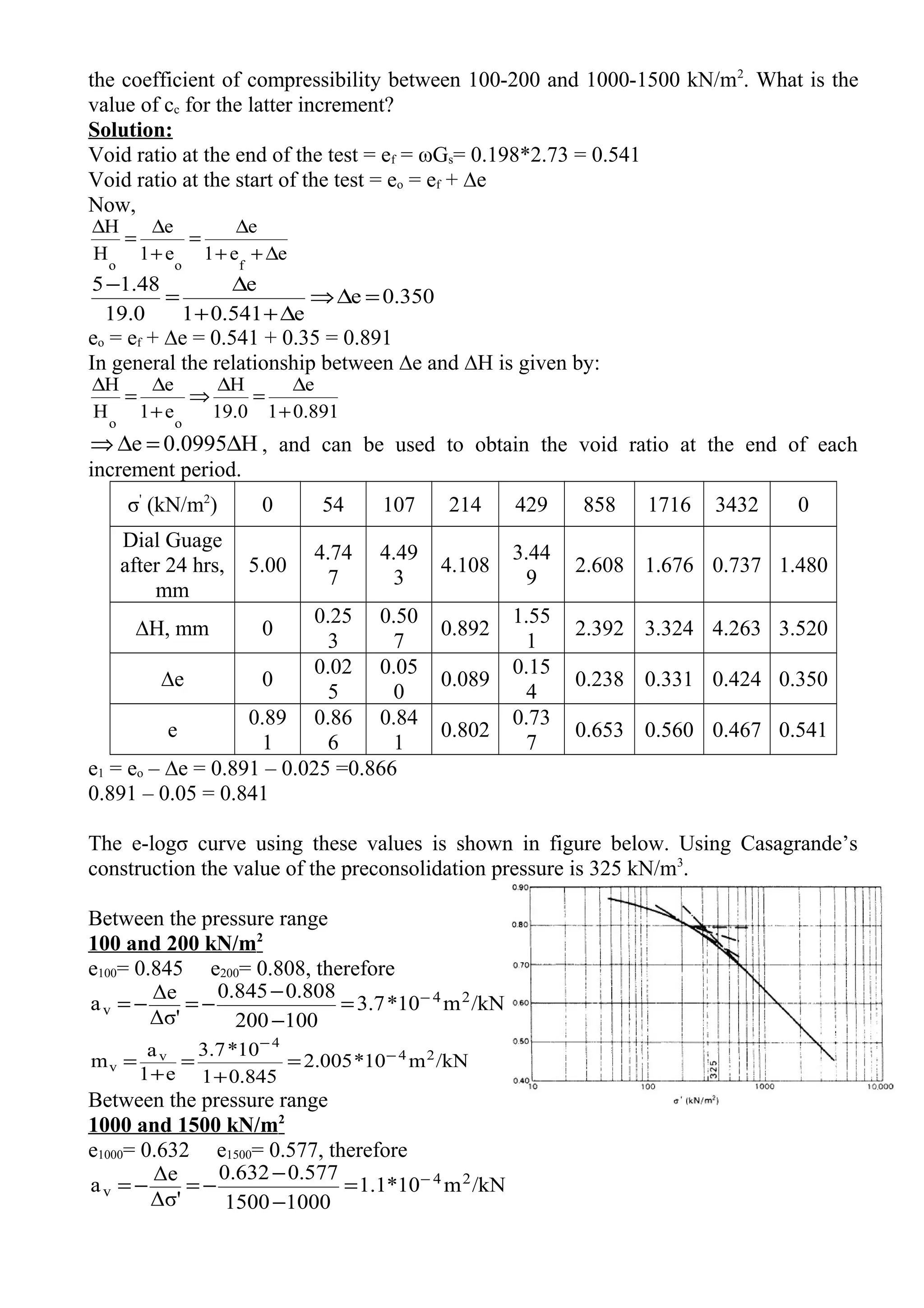
Example 5:
A soil profile shown in figure below, if a uniform distributed load,Δσ , is applied at
the ground surface, what is the settlement of the clay layer caused by primary
consolidation if:
1. The clay is normally consolidated
2. The preconsolidation pressure (σ'c) = 190 kN/m2
3. σ'c = 170 kN/m2
Use cs=1/6 cc
Solution:
1. The clay is normally consolidated
the average effective stress at the middle

5. of the clay layer is
2
o
kN/m79.14
9.81)-2(199.81)-4(1814*2'σ
=
++=
cc = 0.009(LL-10) = 0.009 (40 – 10) = 0.27
o
'
o
o
c
c σ'
σΔσ
log
e1
Hc
S
′+
+
=
mm132m321.0
79.14
10079.14
log
0.81
4*0.27
Sc
==
+
+
=
2. The preconsolidation pressure (σ'c) = 190 kN/m2
2'
o kN/m179.14σΔσ =′+
σ'c = 190 kN/m2
Because 2'
o kN/m179.14σΔσ =′+ < σ'c = 190 kN/m2
o
'
o
o
s
c σ'
σΔσ
log
e1
Hc
S
′+
+
= , cs = 1/6 cc = 1/6 * 0.27 = 0.045
mm36m0.036
79.14
179.14
log
0.81
4*0.045
Sc
==
+
=
3. σ'c = 170 kN/m2
Because '
o
'
c
'
o σσσΔσ >>′+
c
'
o
o
c
o
'
c
o
s
c σ'
σΔσ
log
e1
Hc
σ'
σ
log
e1
Hc
S
′+
+
+
+
=
mm46.9m.04690
170
179.14
log
0.81
4*0.27
179.14
170
log
0.81
4*0.045
Sc
==
+
+
+
=
Example 6:
For the foundation shown, estimate the consolidation settlement.
Solution:
The average effective stress at the middle of the clay layer is
2
o
kN/m52.833
9.81)-(16
2
2.5
9.81)0.5(17.516.5*2.5'σ
=
++= −
Using approximate method to calculate the 'Δσ at
mid-point of clay layer
2
v kN/m445.13
)25.32)(25.31(
1*2*150
z)z)(L(B
qBL
Δσ =
++
=
++
=
Or using m,n method
15.0
25.3
5.0
z
L
m === , and 31.0
25.3
1
z
B
n === f(m,n) = 0.02
2
kN/m124*150*02.0'Δσ ==
1.0
0.5
2.5
Sand
B*L=1m*2m
G.W.T
?=16.5kN/m3
?sat=17.5kN/m
3
Sand
Clay(N.C.)
q=150kN/m
1.5
?sat=16kN/m3
cc=0.32
cs=0.09
eo=0.8
2

6. 1.5
1.5
2.5
Sand
B*L G.W.T
?=15kN/m
3
?sat=18kN/m
3
Sand
Clay(N.C.)
Gs=2.7,LL=38%
?=35%
Q
o
'
o
o
c
c σ'
σΔσ
log
e1
Hc
S
′+
+
=
mm43.8m3804.0
52.833
13.44552.833
log
0.81
2.5*0.32
Sc
==
+
+
=
Example 7:
In the previous example, if the foundation is circular in shape with diameter of 2.5m,
estimate the consolidation settlement.
Solution:
Using approximate method to calculate the 'Δσ at mid point of clay layer
2
2
2
2
2
kN/m355.28
)25.35.2(
5.2*150
Z)(D
qD
σΔ =
+
=
+
=′
or using
2.6
1.25
3.25
R
z
== , and 0
1.25
0
R
x
== from figure 0.18
q
Δσv
≈
2
kN/m27150*18.0σΔ ==′
mm82.9m8290.0
52.833
28.35552.833
log
0.81
2.5*0.32
Sc
==
+
+
=
Example 8:
Refer to figure shown below, given that B=1.5m, L=2.5m, and Q=120 kN. Calculate
the primary consolidation settlement of the foundation.
Solution:
0.945
1
2.7*0.35
S
sωG
eo
===
3
w
s
sat
clay kN/m18.49.81*
0.9451
0.9452.7
γ
e1
eG
γ =
+
+
=
+
+
=
2
o
kN/m5.5234
9.81)-(18.4
2
2.5
9.81)-1.5(1815*1.5'σ
=
++=
'Δσ at the base of the foundation = 2
32kN/m
2.5*1.5
120
=
To determine the net consolidation pressure at mid height of clay layer under the
center of the foundation, the foundation's base must be divided into four equal
0.75*1.25 rectangular areas.
z = 1.5+2.5/2 = 2.75m from the foundation's base
45.0
75.2
25.1
z
L
m === , and 27.0
75.2
75.0
z
B
n === f(m,n) = 0.047
2
kN/m016.64*32*047.0'Δσ ==
2'
o kN/m51.5396.01645.523σΔσ =+=′+
cc = 0.009(LL-10) = 0.009 (38 – 10) = 0.252
o
'
o
o
c
c σ'
σΔσ
log
e1
Hc
S
′+
+
=

7. mm4.17m0174.0
45.523
51.539
log
0.9451
2.5*0.252
Sc
==
+
=
Example 9:
A building is supporting on a raft 45m x 30m, the net foundation pressure being 125
kN/m2
. The soil profile is shown in figure below. The value of mv = 0.35 m2
/MN.
Determine the final settlement under the center of the raft due to consolidation of the
clay.
Solution: at mid point of clay layer,
z = 24 – 3.5 + 2 = 23.5m
96.0
5.23
5.22
z
L
m === , and 64.0
5.23
15
z
B
n === f(m,n) = 0.14
2
kN/m704*125*14.0'Δσ ==
mm98m0.09870*4*10*0.35σHmS 3-
**vc
===′∆=
Example 10:
A stratum of normally loaded clay of 7m thick is located at a depth 12m below
ground level. The (ωn) of the clay is 43% and its LL is 48%. The Gs of the solid particles
is 2.76. the water table is located at a depth of 5m below the ground surface. The soil is
sand above the clay stratum. The submerged unit weight of sand is 11 kN/m3
and the
same weighs 18 kN/m3
above water table. The average increase in pressure at the center
of the clay stratum is 120 kN/m2
due to the weight of a building that will be constructed
on the sand above the clay stratum. Estimate the expected settlement of the structure.
Solution:
1) Determination of e and γsub for clay
s
w
W
W
ω = , kN076.2781.9*76.2*1γGVW wsss ===

8. kN643.11076.27*43.0ωWW sw ===
kN719.38076.27643.11WWW swt =+=+=
187.1
1
76.2*43.0
S
ωG
e s
o
===
3
o
t
t kN/m704.17
187.11
719.38
e1
W
γ =
+
=
+
= , equal to γsat or wsat γ
e1
esG
γ
+
+
=
3
sub kN/m7.8949.8117.704γ =−=
2) Determination of overburden pressure '
oσ
2'
o kN/m194.6293.5*7.8947*1118*5σ =+++=
3) Compression index
cc = 0.009(LL-10) = 0.009(48-10) = 0.342
4) Excess pressure ∆σ' = 120 kN/m2
5) Total Settlement
o
'
o
o
c
c σ'
σΔσ
log
e1
Hc
S
′+
+
=
mm228m228.0
194.629
120194.629
log
1.1871
7*0.342
Sc
==
+
+
=
Example 11:
Soil investigation at a site gave the following information. Top soil up to a depth of
10.6m is fine sand, and below this lies soft clay layer of 7.6m thick. The water table is
at 4.6m below the ground surface. The submerged unit weight of sand is 10.4 kN/m3
,
and wet unit weight above water table is 17.6 kN/m3
. The water content of normally
consolidated clay is 40%, its LL is 45% and Gs is 2.78. The proposed construction will
transmit a net pressure of 120 kN/m2
. Find the average settlement of the clay layer.
Solution:
cc = 0.009(LL-10) = 0.009(45-10) = 0.315
112.1
1
78.2*4.0
S
ωG
e s
o
===
3
wsat kN/m078.189.81*
1.1121
1.1122.78γ
e1
esG
γ =
+
+=
+
+
=
3
sub
kN/m8.2689.8118.078γ =−=
Effective overburden pressure at the mid height of the clay layer is
2'
o kN/m174.7783.8*8.26810.4*617.6*4.6σ =+++=
o
'
o
o
c
c σ'
σΔσ
log
e1
Hc
S
′+
+
=
mm257m257.0
174.778
120174.778
log
1.1121
7.6*0.315
Sc
==
+
+
=
Example 12:
Two points on a curve for normally consolidated clay have the following
coordinates: Point 1: e1 = 0.7, σ1 = 1 kg/cm2

9. Point 2: e2 = 0.6, σ2 = 3 kg/cm2
If the average overburden pressure on a 6m thick clay layer is 1.5 kg/cm2
, how much
settlement the clay layer experience due to additional load intensity of 1.6 kg/cm2
.
Solution:
21.0
13log
6.07.0
σ
σ
log
ee
c
1
2
21
c =
−
=
−
=
We need the initial void ratio eo at an overburden pressure of 1.5 kg/cm2
.
5.1
3
log21.0)6.0e(21.0
σ
σ
log
ee
c o
o
2
2o
c =−⇒=
−
=
0.6630.0630.6eo =+=⇒
o
'
o
o
c
c σ'
σΔσ
log
e1
Hc
S
′+
+
=
mm239m239.0
1.5
1.61.5
log
0.6631
6*0.21
Sc
==
+
+
=
Example 13:
A footing has a size of 3m by 1.5m and it causes a pressure increment of 200 kN/m2
at its base. Determine the consolidation settlement at the middle of the clay layer.
Assume 2:1 pressure distribution.
Solution:
2
'
o
kN/m1.885
5.19*1.58.19*0.516*2.5σ
=
+++=
2
v
kN/m692.27
)5.33)(5.35.1(
3*5.1*200
z)z)(L(B
qBL
Δσ
=
++
=
++
=
o
'
o
o
c
c σ'
σΔσ
log
e1
Hc
S
′+
+
=
mm93m093.0
51.88
27.69251.88
log
0.81
3*0.3
Sc
==
+
+
=

10. Point 2: e2 = 0.6, σ2 = 3 kg/cm2
If the average overburden pressure on a 6m thick clay layer is 1.5 kg/cm2
, how much
settlement the clay layer experience due to additional load intensity of 1.6 kg/cm2
.
Solution:
21.0
13log
6.07.0
σ
σ
log
ee
c
1
2
21
c =
−
=
−
=
We need the initial void ratio eo at an overburden pressure of 1.5 kg/cm2
.
5.1
3
log21.0)6.0e(21.0
σ
σ
log
ee
c o
o
2
2o
c =−⇒=
−
=
0.6630.0630.6eo =+=⇒
o
'
o
o
c
c σ'
σΔσ
log
e1
Hc
S
′+
+
=
mm239m239.0
1.5
1.61.5
log
0.6631
6*0.21
Sc
==
+
+
=
Example 13:
A footing has a size of 3m by 1.5m and it causes a pressure increment of 200 kN/m2
at its base. Determine the consolidation settlement at the middle of the clay layer.
Assume 2:1 pressure distribution.
Solution:
2
'
o
kN/m1.885
5.19*1.58.19*0.516*2.5σ
=
+++=
2
v
kN/m692.27
)5.33)(5.35.1(
3*5.1*200
z)z)(L(B
qBL
Δσ
=
++
=
++
=
o
'
o
o
c
c σ'
σΔσ
log
e1
Hc
S
′+
+
=
mm93m093.0
51.88
27.69251.88
log
0.81
3*0.3
Sc
==
+
+
=