SlideShare a Scribd company logo
1 of 17
Download to read offline
Finite Difference
and
Interpolation
Course- B.Tech
Semester-IV
Subject- ENGINEERING MATHEMATICS-IV
Unit- IV
RAI UNIVERSITY, AHMEDABAD
Unit-IV Finite Difference and Interpolation
Rai University | Ahmedabad
2
Content
Finite differences, difference tables, Newton’s forward interpolation & it’s problems, Newton’s
backward interpolation & it’s problems, stirling's interpolation formula & Problems based on it,
Newton’s divided difference formula for unequal intervals & it’s problems ,Lagrange’s divided
difference formula for unequal intervals & it’s problems
Unit-IV Finite Difference and Interpolation
Rai University | Ahmedabad
3
1.1 Finite differences— Let = ( ) be a function and ∆ = ℎ denote the increment in the
independent variable . Assume that∆ , increment in the argument (also known as the
interval or spacing) is fixed. i.e. ℎ =constant . Then the first finite difference y is defined as—
∆ = ∆ ( ) = ( + ∆ ) − ( )
Similarly finite differences of higher orders are denoted as follows—
∆ = ∆(∆ ) = ∆ ( + ∆ ) − ( )
= ∆ ( + ∆ ) − ∆ ( )
= [ ( + 2∆ ) − ( + ∆ )] − [ ( + ∆ ) − ( )]
∆ = ( + 2∆ ) − 2 ( + ∆ ) + ( )
In general ∆ = ∆(∆ ), for = 2,3,4 …
Now consider the function = ( )specified by the tabulated series = ( ) for a set of
equivalent points where = 0,1,2, … , and ∆ = ∆ − = ℎ =constant. Thus the
tabulated function consists of ordered pairs ( , ), ( , ), … , ( , ), …. Here entries
are known as entries.
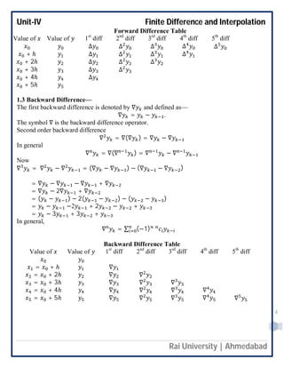
1.2 Forward Difference—
The first forward difference is denoted by ∆ and defined as
∆ = − .
The symbol ∆ is the forward difference operator.
Properties—
1. ∆ = 0 (Differences of constant function are zero)
2. ∆( ) = ∆( ), where is a constant .
3. ∆( + ) = ∆ + ∆
4. ∆( ) = ∆ + ∆
5. ∆ (∆ ) = ∆
6. Where and are non-negative integers and ∆ = (By definition).
7. The higher order forward difference are defined as:
8. The second order forward difference of is
9. ∆ = ∆(∆ ) = ∆ − ∆
In general,
∆ = ∆(∆ ) = ∆ − ∆
It defines the nth
order forward differences.
Any higher order forward differences can be expressed in terms of the successive values of
the function.
Example:
1.
∆ = − 2 +
2.
∆ = − 3 + 3 −
Unit-IV Finite Difference and Interpolation
Rai University | Ahmedabad
4
Forward Difference Table
Value of Value of 1st
diff 2nd
diff 3rd
diff 4th
diff 5th
diff
∆ ∆ ∆ ∆ ∆
+ ℎ ∆ ∆ ∆ ∆
+ 2ℎ ∆ ∆ ∆
+ 3ℎ ∆ ∆
+ 4ℎ ∆
+ 5ℎ
1.3 Backward Difference—
The first backward difference is denoted by ∇ and defined as—
∇ = − .
The symbol ∇ is the backward difference operator.
Second order backward difference
∇ = ∇(∇ ) = ∇ − ∇
In general
∇ = ∇(∇ ) = ∇ − ∇
Now
∇ = ∇ − ∇ = (∇ − ∇ ) − (∇ − ∇ )
= ∇ − ∇ − ∇ + ∇
= ∇ − 2∇ + ∇
= ( − ) − 2( − ) − ( − )
= − −2 + 2 − +
= − 3 + 3 +
In general,
∇ = ∑ (−1)
Backward Difference Table
Value of Value of 1st
diff 2nd
diff 3rd
diff 4th
diff 5th
diff
= + ℎ ∇
= + 2ℎ ∇ ∇
= + 3ℎ ∇ ∇ ∇
= + 4ℎ ∇ ∇ ∇ ∇
= + 5ℎ ∇ ∇ ∇ ∇ ∇
Unit-IV Finite Difference and Interpolation
Rai University | Ahmedabad
5
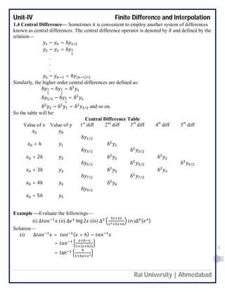
1.4 Central Difference— Sometimes it is convenient to employ another system of differences
known as central differences. The central difference operator is denoted by and defined by the
relation—
− = δ /
− = δ
.
.
.
− = δ ( )/
Similarly, the higher order central differences are defined as:
δ − δ = δ
δ / − δ = δ
δ − δ = δ / and so on.
So the table will be:
Central Difference Table
Value of Value of 1st
diff 2nd
diff 3rd
diff 4th
diff 5th
diff
δ /
+ ℎ δ
δ / δ /
+ 2ℎ δ δ
δ / δ / δ /
+ 3ℎ δ δ
δ / δ /
+ 4ℎ δ
δ /
+ 5ℎ
Example —Evaluate the followings—
(i) ∆ (ii) ∆ log 2 (iii) ∆ (iv)∆ ( )
Solution—
(i) ∆ = ( + ℎ) −
= ( )
= tan
Unit-IV Finite Difference and Interpolation
Rai University | Ahmedabad
6
(ii) ∆ log 2 = log 2( + ℎ) − log 2
= log 2( + ℎ) − log 2 + log 2 − log 2
= [log 2( + ℎ) − log 2 ] + [ − ] log 2
= log
+ ℎ
+ [ − 1] log 2
= log 1 +
ℎ
+ ( − 1) log 2
(iii) ∆ = ∆ ( )( )
= ∆ +
= ∆ ∆ + ∆
= ∆ 2 − + 3 −
= 2∆ ( )( )
+3∆ ( )( )
= −2∆ ( )( )
−3∆ ( )( )
= −2 ( )( )
− ( )( )
− 3 ( )( )
− ( )( )
= ( )( )( )
+ ( )( )( )
=
( ) ( )
( )( )( )( )
= ( )( )( )( )
= ( )( )( )( )
=
( )
( )( )( )( )
(iv) ∆ ( ) = − = ( − 1)
∆ ( ) = ∆ (∆ ) = ∆[( − 1) ] = ( − 1)∆ = ( − 1)( − 1)
∆ ( ) = ( − 1)
∆ ( ) = ( − 1)
∆ ( ) = ( − 1)
⋮
∆ ( ) = ( − 1) .
1.5 Difference of a polynomial— The nth
difference of the nth -
degree polynomial are constant
and all higher order differences are zero.
Let the polynomial of nth
degree in is:
( ) = + + … + ( + ℎ) +
∆ ( ) = ( + ℎ) − ( )
= [( + ℎ) − ] + [( + ℎ) − ] + ⋯ + ℎ
= ℎ + + + ⋯ + + ′
Where , , … , ′ are new constants.
Thus the first difference of a polynomial of nth -
degree is a polynomial of degree ( − 1).
Unit-IV Finite Difference and Interpolation
Rai University | Ahmedabad
7
Similarly
∆ ( ) = ∆[ ( + ℎ) − ( )] = ∆ ( + ℎ) − ∆ ( )
= ℎ[( + ℎ) − ] + [( + ℎ) − ] + ⋯ + ℎ
= ( − 1)ℎ + + + ⋯ + ′′
∴ the second differences represent a polynomial of degree ( − 2).
Continuing in this process for the nth differences we get a polynomial of degree zero.
i.e. ∆ ( ) = ( − 1)( − 2) … 1
ℎ = ! ℎ , which is constant.
Hence the ( + 1)th
and higher order differences of a polynomial of nth
degree will be zero.
Example— Evaluate ∆ [(1 − )(1 − )(1 − )(1 − )].
Solution— ∆ [(1 − )(1 − )(1 − )(1 − )]
= ∆ [ + (. . . ) + (… ) + ⋯ + 1]
= (10!) [∵ ∆ ( ) = 0 < 10]
Example— Find the missing value of the following table:
: 45 50 55 60 65
: 3.0 _______ 2.0 ________ -2.4
Solution—The difference is –
∆ ∆ ∆
45 = 3.0 − 3 5 − 2 3 + − 9
50 2 − + − 4 3.6 − − 3
55 = 2.0 − 2 −0.4 − 2
60 −2.4 −
65 = −2.4
Solving the two equations 3 + − 9 = 0 and 3.6 − − 3 = 0.
we can find the value of and .
3 + = 9 … ( )
+ 3 = 3.6 … ( )
From ( )
= 9 − 3 .
Substituting the value of ( )
+ 3(9 − 3 ) = 3.6
⟹ −8 = 3.6 − 27
⟹ =
−23.4
−8
= 2.935
= 9 − 3(2.935) = 9 − 8.775 = 0.225.
Unit-IV Finite Difference and Interpolation
Rai University | Ahmedabad
8
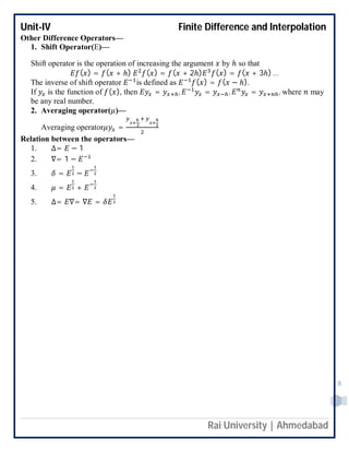
Other Difference Operators—
1. Shift Operator(E)—
Shift operator is the operation of increasing the argument by ℎ so that
( ) = ( + ℎ) ( ) = ( + 2ℎ) ( ) = ( + 3ℎ) …
The inverse of shift operator is defined as ( ) = ( − ℎ).
If is the function of ( ), then = , = , = , where may
be any real number.
2. Averaging operator( )—
Averaging operator =
Relation between the operators—
1. ∆= − 1
2. ∇= 1 −
3. = −
4. = +
5. ∆= ∇= ∇ =
Unit-IV Finite Difference and Interpolation
Rai University | Ahmedabad
9
2.1 Interpolation—Let = ( ) is tabulated for the equally spaced values of
= , , , … , , where = + ℎ, = 0,1,2, … ,
⟹ = + ℎ,
= + 2ℎ
= + 3ℎ
= + ℎ
It gives— = , , ,… ,
…
…
The process of finding the values of corresponding to any value of = between and
is called interpolation.
The study of interpolation is based on the concept of difference of a function.
To determine the values of ( ) of ′( ) for some intermediate values of various types of
difference are very much useful.
2.2 Newton’s forward difference interpolation— Let the function = ( ) takes the values
, , ,… corresponding to the values , + ℎ, + 2ℎ, … of . Suppose it is required to
evaluate ( ) for = + ℎ, where is any real number.
For any real number , we have defined such that—
( ) = ( + ℎ)
= ( + ℎ) = ( ) = (1 + ∆) [∵ = 1 +△]
= 1 + △ +
( )
!
△ +
( )( )
!
△ + ⋯ [Binomial theorem]
= + △ +
( )
!
△ +
( )( )
!
△ + ⋯ … (1)
It is called Newton’s forward difference interpolation formula as (1) contains and the
forward differences of .
2.3 Newton’s backward difference interpolation— Let the function = ( ) takes the
values , , ,… corresponding to the values , + ℎ, + 2ℎ, … of . Suppose it is
required to evaluate ( ) for
= + ℎ, where is any real number.
Then we have
= ( + ℎ) = ( ) = (1 − ∇) [∵ = 1 − ∇]
= 1 + ∇ +
( )
!
∇ +
( )( )
!
∇ + ⋯ [ ℎ ]
= + ∇ +
( )
!
∇ +
( )( )
!
∇ + ⋯ … (2)
It is called Newton’s forward difference interpolation formula as eq (1) contains and the
forward differences of .
Unit-IV Finite Difference and Interpolation
Rai University | Ahmedabad
10
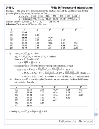
Example—The table gives the distances in the nautical miles of the visible horizon for the
given heights in feet above the earth’s surface:
=height : 100 150 200 250 300 350 400
=distance: 10.63 13.03 15.04 16.81 18.42 19.90 21.27
Find the value of , when ( ) = 218 ( ) 410 .
Solution—The forward difference table is—
∆ ∆ ∆ ∆
100 10.63
150 13.03 2.40
200 15.04 2.01 -0.39
250 16.81 1.77 -0.24 0.15
300 18.42 1.61 -0.16 0.08 -0.07
350 19.90 1.48 -0.13 0.03 -0.05
400 21.27 1.37 -0.11 0.02 -0.01
(i) For = 200, = 15.04
∆ = 1.77, ∆ = −0.16, ∆ = 0.03etc.
Since = 218 and ℎ = 50
∴ = = = 0.36
Using Newton’s forward difference interpolation formula we get
= + △ +
( )
!
△ +
( )( )
!
△ + ⋯
= 15.04 + 0.36(1.77) +
. ( . )
(−0.16) +
. ( . )( . )
(0.03) + ⋯
= 15.04 + 0.637 + 0.018 + 0.001 + ⋯ = 15.696 i.e. 15.7 nautical miles.
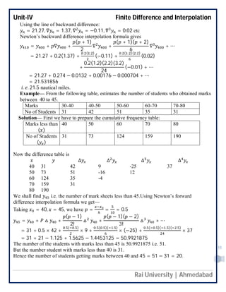
(ii) Since = 410 is near the end of the table, we use Newton’s backward difference
interpolation formula.
∇ ∇ ∇ ∇
100 10.63 2.40 -0.39 0.15 -0.07
150 13.03 2.01 -0.24 0.08 -0.05
200 15.04 1.77 -0.16 0.03 -0.01
250 16.81 1.61 -0.13 0.02
300 18.42 1.48 -0.11
350 19.90 1.37
400 21.27
∴ Taking = 400, = = = 0.2
Unit-IV Finite Difference and Interpolation
Rai University | Ahmedabad
11
Using the line of backward difference:
= 21.27, ∇ = 1.37, ∇ = −0.11, ∇ = 0.02 etc
Newton’s backward difference interpolation formula gives
= + ∇ +
( + 1)
2
∇ +
( + 1)( + 2)
6
∇ + ⋯
= 21.27 + 0.2(1.37) +
. ( . )
(−0.11) +
. ( . )( . )
(0.02)
+
0.2(1.2)(2.2)(3.2)
24
(−0.01) + ⋯
= 21.27 + 0.274 − 0.0132 + 0.00176 − 0.000704 + ⋯
= 21.531856
. . 21.5 nautical miles.
Example— From the following table, estimates the number of students who obtained marks
between 40 to 45.
Marks 30-40 40-50 50-60 60-70 70-80
No of Students 31 42 51 35 31
Solution— First we have to prepare the cumulative frequency table:
Marks less than
( )
40 50 60 70 80
No of Students
( )
31 73 124 159 190
Now the difference table is
∆ ∆ ∆ ∆
40 31 42 9 -25 37
50 73 51 -16 12
60 124 35 -4
70 159 31
80 190
We shall find i.e. the number of mark sheets less than 45.Using Newton’s forward
difference interpolation formula we get—
Taking = 40, = 45, we have = = = 0.5
= + △ +
( − 1)
2!
△ +
( − 1)( − 2)
3!
△ + ⋯
= 31 + 0.5 × 42 +
. ( . )
× 9 +
. ( . )( . )
× (−25) +
. ( . )( . )( . )
× 37
= 31 + 21 − 1.125 + 1.5625 − 1.4453125 = 50.9921875
The number of the students with marks less than 45 is 50.9921875 i.e. 51.
But the number student with marks less than 40 is 31.
Hence the number of students getting marks between 40 and 45 = 51 − 31 = 20.
Unit-IV Finite Difference and Interpolation
Rai University | Ahmedabad
12
2.4 Central Difference Interpolation Formulae— If takes the values − 2ℎ, −
ℎ, , + ℎ, + 2ℎ are the corresponding values of = ( ) are , , , , , then we
write the difference table as:
Value of Value of 1st
diff 2nd
diff 3rd
diff 4th
diff
− 2ℎ
∆ (= δ / )
− ℎ ∆ (= δ )
∆ (= δ / ) ∆ (= δ )
∆ (= δ ) ∆ (= δ )
∆ (= δ / ) ∆ (= δ )
+ ℎ ∆ (= δ )
∆ (= δ / )
+ 2ℎ
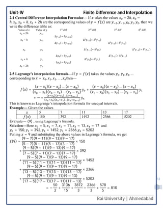
2.5 Lagrange’s interpolation formula—If = ( ) takes the values , , , …
corresponding to = , , , … , then—
( ) =
( − )( − ) … ( − )
( − )( − ) … ( − )
+
( − )( − ) … ( − )
( − )( − ) … ( − )
+ ⋯ +
( )( )…( )
( )( )…( )
This is known as Lagrange’s interpolation formula for unequal intervals.
Example— Given the values
5 7 11 13 17
( ) 150 392 1492 2366 5202
Evaluate— (9) , using Lagrange’s formula.
Solution—Here = 5, = 7, = 11, = 13, = 17 and
= 150, = 392, = 1452, = 2366, = 5202
Putting = 9 and substituting the above values in Lagrange’s formula, we get
(9) =
(9 − 7)(9 − 11)(9 − 13)(9 − 17)
(5 − 7)(5 − 11)(5 − 13)(3 − 17)
× 150
+
(9 − 5)(9 − 11)(9 − 13)(9 − 17)
(7 − 5)(7 − 11)(7 − 13)(7 − 17)
× 392
+
(9 − 5)(9 − 7)(9 − 13)(9 − 17)
(11 − 5)(11 − 7)(11 − 13)(11 − 17)
× 1452
+
(9 − 5)(9 − 7)(9 − 11)(9 − 17)
(13 − 5)(13 − 7)(13 − 11)(13 − 17)
× 2366
+
(9 − 5)(9 − 7)(9 − 11)(9 − 13)
(17 − 5)(17 − 7)(17 − 11)(17 − 13)
× 5202
= −
50
2
+
3136
15
+
3872
3
−
2366
3
+
578
5
= 810
Unit-IV Finite Difference and Interpolation
Rai University | Ahmedabad
13
2.6 Divided difference—
TheLagrange’s formula has the drawback that if another interpolation areinterested then the
interpolation coefficient are required to recalculate.
This problem is solved in Newton’s divided difference interpolation formula.
If ( , ), ( , ), ( , ) … be given points, then the first divided difference for the argument
is , is defined by the relation [ , ] = .
Similarly,
[ , ] = and[ , ] = etc.
The second divided difference for the argument is , , is defined as [ , , ] =
[ ] [ , ]
.
The third divided difference for the argument is , , , is defined as [ , , , ] =
[ , , ] [ , , ]
and so on.
2.7 Newton’s divided difference interpolation formula— Let , , , … be the values of
= ( ) corresponding to the arguments , , , … , . Then from the definition of divided
differences, we have [ , ] =
= +( − )[ − ] … ( )
Again, [ , , ] =
[ , ] [ , ]
Which give—
[ , ] = [ , ] +( − ) + ( − ) [ , , ]
Substituting this values in the eq(i), we get
= +( − )[ − ] + ( − )( − ) [ , , ] … ( )
Also, [ , , , ] =
[ , , ] [ , , ]
Which gives [ , , ] = [ , , ] −( , )[ , , , ]
Substituting this values of [ , , ] in the eq(ii), we obtain
= +( − )[ − ] + ( − )( − ) [ , , ]
+( − )( − ) ( − )[ , , , ]
Proceeding in this way, we get
= +( − )[ − ] + ( − )( − ) [ , , ]
+( − )( − )( − )[ , , , ] + ⋯
+( − )( − ) … ( − )[ , , , … , ] … ( )
This is called as Newton’s divided difference interpolation formula.
Unit-IV Finite Difference and Interpolation
Rai University | Ahmedabad
14
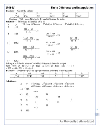
Example— Given the values
5 7 11 13 17
( ) 150 392 1492 2366 5202
Evaluate (9) , using Newton’s divided difference formula.
Solution—The divided difference table is:
1st
divided difference 2nd
divided difference 3rd
divided difference
5 150
392 − 150
7 − 5
= 121
7 392 265 − 121
11 − 5
= 24
1452 − 392
11 − 7
= 265
32 − 24
13 − 5
= 1
11 1452 457 − 265
13 − 7
= 32
2366 − 1452
13 − 11
= 457
42 − 32
17 − 7
= 1
13 2366 709 − 457
17 − 11
= 42
5202 − 2366
17 − 13
= 709
17 5202
Taking = 9 in the Newton’s divided difference formula, we get
(9) = 150 + (9 − 5) × 121 + (9 − 5)(9 − 7) × 24 + (9 − 5)(9 − 7)(9 − 11) × 1
= 150 + 484 + 192 − 16 = 810
Example—Determine ( ) as a polynomial in nfor the following data:
−4 −1 0 2 5
( ) 1245 33 5 9 1335
Solution—
1st
divided
difference
2nd
divided
difference
3rd
divided
difference
4th
divided
difference
−4 1245
−404
−1 33 94
−28 −14
0 5 10 3
2 13
2 9 88
442
5 1335
Unit-IV Finite Difference and Interpolation
Rai University | Ahmedabad
15
Applying Newton’s divided difference formula—
( ) = ( ) + 0 +( − )[ − ] + ( − )( − ) [ , , ] + ⋯
= 1245 + ( + 4)(−404) + ( + 4)( + 1)(94)
+( + 4)( + 1)( − 0)(−14) + ( + 4) ( + 1)( − 2)(3)
= 3 + 5 + 6 − 14 + 5
Unit-IV Finite Difference and Interpolation
Rai University | Ahmedabad
16
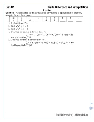
Exercise
Question—Assuming that the following values of belong to a polynomial of degree 4,
compute the next three values:
: 0 1 2 3 4 5 6 7
: 1 -1 1 -1 1 _____ _____ _____
1. Evaluate ∆ 2 .
2. Find ∆ at = 0.
3. Find ∆ at = 0.
4. Construct an forward difference table for
(1) = 1, (2) = 3, (3) = 8, (4) = 15, (5) = 25
and hence find ∆ (1).
5. Construct a central difference table for
(0) = 8, (1) = 12, (2) = 20, (3) = 34, (4) = 60
And hence, find (2).
Unit-IV Finite Difference and Interpolation
Rai University | Ahmedabad
17
Reference
1. http://en.wikipedia.org/wiki/File:Finite_Differences.svg
2. Higher Engineering Mathematics, B.S. Grewal, Khanna Publishers.

More Related Content

What's hot

Finite difference method
Finite difference methodFinite difference method
Finite difference methodDivyansh Verma
 
Interpolation and its applications
Interpolation and its applicationsInterpolation and its applications
Interpolation and its applicationsRinkuMonani
 
Linear differential equation
Linear differential equationLinear differential equation
Linear differential equationPratik Sudra
 
Partial differential equations
Partial differential equationsPartial differential equations
Partial differential equationsaman1894
 
Numerical solution of ordinary differential equation
Numerical solution of ordinary differential equationNumerical solution of ordinary differential equation
Numerical solution of ordinary differential equationDixi Patel
 
Engineering Mathematics-IV_B.Tech_Semester-IV_Unit-V
Engineering Mathematics-IV_B.Tech_Semester-IV_Unit-VEngineering Mathematics-IV_B.Tech_Semester-IV_Unit-V
Engineering Mathematics-IV_B.Tech_Semester-IV_Unit-VRai University
 
Gauss Forward And Backward Central Difference Interpolation Formula
 Gauss Forward And Backward Central Difference Interpolation Formula  Gauss Forward And Backward Central Difference Interpolation Formula
Gauss Forward And Backward Central Difference Interpolation Formula Deep Dalsania
 
Newton's forward & backward interpolation
Newton's forward & backward interpolationNewton's forward & backward interpolation
Newton's forward & backward interpolationHarshad Koshti
 
Homogeneous Linear Differential Equations
 Homogeneous Linear Differential Equations Homogeneous Linear Differential Equations
Homogeneous Linear Differential EquationsAMINULISLAM439
 
Linear differential equation with constant coefficient
Linear differential equation with constant coefficientLinear differential equation with constant coefficient
Linear differential equation with constant coefficientSanjay Singh
 
Heaviside's function
Heaviside's functionHeaviside's function
Heaviside's functionSeanPereira2
 
presentation on Euler and Modified Euler method ,and Fitting of curve
presentation on Euler and Modified Euler method ,and Fitting of curve presentation on Euler and Modified Euler method ,and Fitting of curve
presentation on Euler and Modified Euler method ,and Fitting of curve Mukuldev Khunte
 
Numerical method for solving non linear equations
Numerical method for solving non linear equationsNumerical method for solving non linear equations
Numerical method for solving non linear equationsMdHaque78
 
Maths-->>Eigenvalues and eigenvectors
Maths-->>Eigenvalues and eigenvectorsMaths-->>Eigenvalues and eigenvectors
Maths-->>Eigenvalues and eigenvectorsJaydev Kishnani
 

What's hot (20)

Finite difference method
Finite difference methodFinite difference method
Finite difference method
 
Interpolation and its applications
Interpolation and its applicationsInterpolation and its applications
Interpolation and its applications
 
Linear differential equation
Linear differential equationLinear differential equation
Linear differential equation
 
Partial differential equations
Partial differential equationsPartial differential equations
Partial differential equations
 
Fourier series
Fourier seriesFourier series
Fourier series
 
Numerical solution of ordinary differential equation
Numerical solution of ordinary differential equationNumerical solution of ordinary differential equation
Numerical solution of ordinary differential equation
 
Engineering Mathematics-IV_B.Tech_Semester-IV_Unit-V
Engineering Mathematics-IV_B.Tech_Semester-IV_Unit-VEngineering Mathematics-IV_B.Tech_Semester-IV_Unit-V
Engineering Mathematics-IV_B.Tech_Semester-IV_Unit-V
 
Gauss sediel
Gauss sedielGauss sediel
Gauss sediel
 
Gauss Forward And Backward Central Difference Interpolation Formula
 Gauss Forward And Backward Central Difference Interpolation Formula  Gauss Forward And Backward Central Difference Interpolation Formula
Gauss Forward And Backward Central Difference Interpolation Formula
 
Group Theory
Group TheoryGroup Theory
Group Theory
 
Newton's forward & backward interpolation
Newton's forward & backward interpolationNewton's forward & backward interpolation
Newton's forward & backward interpolation
 
Homogeneous Linear Differential Equations
 Homogeneous Linear Differential Equations Homogeneous Linear Differential Equations
Homogeneous Linear Differential Equations
 
Linear differential equation with constant coefficient
Linear differential equation with constant coefficientLinear differential equation with constant coefficient
Linear differential equation with constant coefficient
 
Heaviside's function
Heaviside's functionHeaviside's function
Heaviside's function
 
presentation on Euler and Modified Euler method ,and Fitting of curve
presentation on Euler and Modified Euler method ,and Fitting of curve presentation on Euler and Modified Euler method ,and Fitting of curve
presentation on Euler and Modified Euler method ,and Fitting of curve
 
Numerical method for solving non linear equations
Numerical method for solving non linear equationsNumerical method for solving non linear equations
Numerical method for solving non linear equations
 
Rolles theorem
Rolles theoremRolles theorem
Rolles theorem
 
Double Integrals
Double IntegralsDouble Integrals
Double Integrals
 
Fourier series
Fourier seriesFourier series
Fourier series
 
Maths-->>Eigenvalues and eigenvectors
Maths-->>Eigenvalues and eigenvectorsMaths-->>Eigenvalues and eigenvectors
Maths-->>Eigenvalues and eigenvectors
 

Viewers also liked

Engineering Mathematics-IV_B.Tech_Semester-IV_Unit-III
Engineering Mathematics-IV_B.Tech_Semester-IV_Unit-IIIEngineering Mathematics-IV_B.Tech_Semester-IV_Unit-III
Engineering Mathematics-IV_B.Tech_Semester-IV_Unit-IIIRai University
 
Engineering Mathematics-IV_B.Tech_Semester-IV_Unit-I
Engineering Mathematics-IV_B.Tech_Semester-IV_Unit-IEngineering Mathematics-IV_B.Tech_Semester-IV_Unit-I
Engineering Mathematics-IV_B.Tech_Semester-IV_Unit-IRai University
 
Engineering Mathematics-IV_B.Tech_Semester-IV_Unit-II
Engineering Mathematics-IV_B.Tech_Semester-IV_Unit-IIEngineering Mathematics-IV_B.Tech_Semester-IV_Unit-II
Engineering Mathematics-IV_B.Tech_Semester-IV_Unit-IIRai University
 
Mba Ebooks ! Edhole
Mba Ebooks ! EdholeMba Ebooks ! Edhole
Mba Ebooks ! EdholeEdhole.com
 
B.tech semester i-unit-iv_matrices and determinants
B.tech semester i-unit-iv_matrices and determinantsB.tech semester i-unit-iv_matrices and determinants
B.tech semester i-unit-iv_matrices and determinantsRai University
 
M1 unit vi-jntuworld
M1 unit vi-jntuworldM1 unit vi-jntuworld
M1 unit vi-jntuworldmrecedu
 
ECNG 3015 Industrial and Commercial Electrical Systems
ECNG 3015   Industrial and Commercial Electrical SystemsECNG 3015   Industrial and Commercial Electrical Systems
ECNG 3015 Industrial and Commercial Electrical SystemsChandrabhan Sharma
 
Analysis of unsymmetrical faults using bus impedence matrix
Analysis of unsymmetrical faults using bus impedence matrixAnalysis of unsymmetrical faults using bus impedence matrix
Analysis of unsymmetrical faults using bus impedence matrixTrupesh Rupareliya
 
advanced engineering mathematics chapter1.1 solution
advanced engineering mathematics chapter1.1 solutionadvanced engineering mathematics chapter1.1 solution
advanced engineering mathematics chapter1.1 solutionrohit kumar
 
Power system analysis material -Mathankumar.s VMKVEC
Power system analysis material -Mathankumar.s  VMKVECPower system analysis material -Mathankumar.s  VMKVEC
Power system analysis material -Mathankumar.s VMKVECMathankumar S
 
BSC_COMPUTER _SCIENCE_UNIT-5_DISCRETE MATHEMATICS
BSC_COMPUTER _SCIENCE_UNIT-5_DISCRETE MATHEMATICSBSC_COMPUTER _SCIENCE_UNIT-5_DISCRETE MATHEMATICS
BSC_COMPUTER _SCIENCE_UNIT-5_DISCRETE MATHEMATICSRai University
 
B.tech ii unit-4 material vector differentiation
B.tech ii unit-4 material vector differentiationB.tech ii unit-4 material vector differentiation
B.tech ii unit-4 material vector differentiationRai University
 
BSC_Computer Science_Discrete Mathematics_Unit-I
BSC_Computer Science_Discrete Mathematics_Unit-IBSC_Computer Science_Discrete Mathematics_Unit-I
BSC_Computer Science_Discrete Mathematics_Unit-IRai University
 
Btech_II_ engineering mathematics_unit5
Btech_II_ engineering mathematics_unit5Btech_II_ engineering mathematics_unit5
Btech_II_ engineering mathematics_unit5Rai University
 
B.tech ii unit-5 material vector integration
B.tech ii unit-5 material vector integrationB.tech ii unit-5 material vector integration
B.tech ii unit-5 material vector integrationRai University
 

Viewers also liked (20)

Engineering Mathematics-IV_B.Tech_Semester-IV_Unit-III
Engineering Mathematics-IV_B.Tech_Semester-IV_Unit-IIIEngineering Mathematics-IV_B.Tech_Semester-IV_Unit-III
Engineering Mathematics-IV_B.Tech_Semester-IV_Unit-III
 
Engineering Mathematics-IV_B.Tech_Semester-IV_Unit-I
Engineering Mathematics-IV_B.Tech_Semester-IV_Unit-IEngineering Mathematics-IV_B.Tech_Semester-IV_Unit-I
Engineering Mathematics-IV_B.Tech_Semester-IV_Unit-I
 
Engineering Mathematics-IV_B.Tech_Semester-IV_Unit-II
Engineering Mathematics-IV_B.Tech_Semester-IV_Unit-IIEngineering Mathematics-IV_B.Tech_Semester-IV_Unit-II
Engineering Mathematics-IV_B.Tech_Semester-IV_Unit-II
 
Mba Ebooks ! Edhole
Mba Ebooks ! EdholeMba Ebooks ! Edhole
Mba Ebooks ! Edhole
 
B.tech semester i-unit-iv_matrices and determinants
B.tech semester i-unit-iv_matrices and determinantsB.tech semester i-unit-iv_matrices and determinants
B.tech semester i-unit-iv_matrices and determinants
 
M1 unit vi-jntuworld
M1 unit vi-jntuworldM1 unit vi-jntuworld
M1 unit vi-jntuworld
 
ECNG 3015 Industrial and Commercial Electrical Systems
ECNG 3015   Industrial and Commercial Electrical SystemsECNG 3015   Industrial and Commercial Electrical Systems
ECNG 3015 Industrial and Commercial Electrical Systems
 
Analysis of unsymmetrical faults using bus impedence matrix
Analysis of unsymmetrical faults using bus impedence matrixAnalysis of unsymmetrical faults using bus impedence matrix
Analysis of unsymmetrical faults using bus impedence matrix
 
advanced engineering mathematics chapter1.1 solution
advanced engineering mathematics chapter1.1 solutionadvanced engineering mathematics chapter1.1 solution
advanced engineering mathematics chapter1.1 solution
 
Power system analysis material -Mathankumar.s VMKVEC
Power system analysis material -Mathankumar.s  VMKVECPower system analysis material -Mathankumar.s  VMKVEC
Power system analysis material -Mathankumar.s VMKVEC
 
BSC_COMPUTER _SCIENCE_UNIT-5_DISCRETE MATHEMATICS
BSC_COMPUTER _SCIENCE_UNIT-5_DISCRETE MATHEMATICSBSC_COMPUTER _SCIENCE_UNIT-5_DISCRETE MATHEMATICS
BSC_COMPUTER _SCIENCE_UNIT-5_DISCRETE MATHEMATICS
 
B.tech ii unit-4 material vector differentiation
B.tech ii unit-4 material vector differentiationB.tech ii unit-4 material vector differentiation
B.tech ii unit-4 material vector differentiation
 
B.Tech-II_Unit-IV
B.Tech-II_Unit-IVB.Tech-II_Unit-IV
B.Tech-II_Unit-IV
 
B.Tech-II_Unit-I
B.Tech-II_Unit-IB.Tech-II_Unit-I
B.Tech-II_Unit-I
 
BSC_Computer Science_Discrete Mathematics_Unit-I
BSC_Computer Science_Discrete Mathematics_Unit-IBSC_Computer Science_Discrete Mathematics_Unit-I
BSC_Computer Science_Discrete Mathematics_Unit-I
 
merged_document
merged_documentmerged_document
merged_document
 
Btech_II_ engineering mathematics_unit5
Btech_II_ engineering mathematics_unit5Btech_II_ engineering mathematics_unit5
Btech_II_ engineering mathematics_unit5
 
B.tech ii unit-5 material vector integration
B.tech ii unit-5 material vector integrationB.tech ii unit-5 material vector integration
B.tech ii unit-5 material vector integration
 
Unit 1 Introduction
Unit 1 IntroductionUnit 1 Introduction
Unit 1 Introduction
 
B.Tech-II_Unit-V
B.Tech-II_Unit-VB.Tech-II_Unit-V
B.Tech-II_Unit-V
 

Similar to FINITE DIFFERENCE AND INTERPOLATION TECHNIQUES

Matlab lab manual
Matlab lab manualMatlab lab manual
Matlab lab manualnmahi96
 
Study Material Numerical Differentiation and Integration
Study Material Numerical Differentiation and IntegrationStudy Material Numerical Differentiation and Integration
Study Material Numerical Differentiation and IntegrationMeenakshisundaram N
 
engineeringmathematics-iv_unit-v
engineeringmathematics-iv_unit-vengineeringmathematics-iv_unit-v
engineeringmathematics-iv_unit-vKundan Kumar
 
engineeringmathematics-iv_unit-ii
engineeringmathematics-iv_unit-iiengineeringmathematics-iv_unit-ii
engineeringmathematics-iv_unit-iiKundan Kumar
 
Diploma_Semester-II_Advanced Mathematics_Indefinite integration
Diploma_Semester-II_Advanced Mathematics_Indefinite integrationDiploma_Semester-II_Advanced Mathematics_Indefinite integration
Diploma_Semester-II_Advanced Mathematics_Indefinite integrationRai University
 
BCA_MATHEMATICS-I_Unit-V
BCA_MATHEMATICS-I_Unit-VBCA_MATHEMATICS-I_Unit-V
BCA_MATHEMATICS-I_Unit-VRai University
 
Complex differentiation contains analytic function.pptx
Complex differentiation contains analytic function.pptxComplex differentiation contains analytic function.pptx
Complex differentiation contains analytic function.pptxjyotidighole2
 
Module For Mathematics
Module For Mathematics Module For Mathematics
Module For Mathematics jrbt2014
 
Forward & Backward Differenece Table
Forward & Backward Differenece TableForward & Backward Differenece Table
Forward & Backward Differenece TableSaloni Singhal
 
3. DERIVATIVE BY INCREMENT IN CALULUS 01
3. DERIVATIVE BY INCREMENT IN CALULUS 013. DERIVATIVE BY INCREMENT IN CALULUS 01
3. DERIVATIVE BY INCREMENT IN CALULUS 01oliverosmarcial24
 
Applications of Differential Calculus in real life
Applications of Differential Calculus in real life Applications of Differential Calculus in real life
Applications of Differential Calculus in real life OlooPundit
 
Chapter 3 finite difference calculus (temporarily)
Chapter 3 finite difference calculus (temporarily)Chapter 3 finite difference calculus (temporarily)
Chapter 3 finite difference calculus (temporarily)MichaelDang47
 
Numerical Solution Of Delay Differential Equations Using The Adomian Decompos...
Numerical Solution Of Delay Differential Equations Using The Adomian Decompos...Numerical Solution Of Delay Differential Equations Using The Adomian Decompos...
Numerical Solution Of Delay Differential Equations Using The Adomian Decompos...theijes
 
Lesson 21: More Algebra
Lesson 21: More AlgebraLesson 21: More Algebra
Lesson 21: More AlgebraKevin Johnson
 
Notes on Equation of Plane
Notes on Equation of PlaneNotes on Equation of Plane
Notes on Equation of PlaneHerbert Mujungu
 

Similar to FINITE DIFFERENCE AND INTERPOLATION TECHNIQUES (20)

Matlab lab manual
Matlab lab manualMatlab lab manual
Matlab lab manual
 
Study Material Numerical Differentiation and Integration
Study Material Numerical Differentiation and IntegrationStudy Material Numerical Differentiation and Integration
Study Material Numerical Differentiation and Integration
 
doc
docdoc
doc
 
engineeringmathematics-iv_unit-v
engineeringmathematics-iv_unit-vengineeringmathematics-iv_unit-v
engineeringmathematics-iv_unit-v
 
engineeringmathematics-iv_unit-ii
engineeringmathematics-iv_unit-iiengineeringmathematics-iv_unit-ii
engineeringmathematics-iv_unit-ii
 
Diploma_Semester-II_Advanced Mathematics_Indefinite integration
Diploma_Semester-II_Advanced Mathematics_Indefinite integrationDiploma_Semester-II_Advanced Mathematics_Indefinite integration
Diploma_Semester-II_Advanced Mathematics_Indefinite integration
 
Unit iv
Unit ivUnit iv
Unit iv
 
BCA_MATHEMATICS-I_Unit-V
BCA_MATHEMATICS-I_Unit-VBCA_MATHEMATICS-I_Unit-V
BCA_MATHEMATICS-I_Unit-V
 
Complex differentiation contains analytic function.pptx
Complex differentiation contains analytic function.pptxComplex differentiation contains analytic function.pptx
Complex differentiation contains analytic function.pptx
 
Maths digital text
Maths digital textMaths digital text
Maths digital text
 
Module For Mathematics
Module For Mathematics Module For Mathematics
Module For Mathematics
 
Forward & Backward Differenece Table
Forward & Backward Differenece TableForward & Backward Differenece Table
Forward & Backward Differenece Table
 
3. DERIVATIVE BY INCREMENT IN CALULUS 01
3. DERIVATIVE BY INCREMENT IN CALULUS 013. DERIVATIVE BY INCREMENT IN CALULUS 01
3. DERIVATIVE BY INCREMENT IN CALULUS 01
 
Applications of Differential Calculus in real life
Applications of Differential Calculus in real life Applications of Differential Calculus in real life
Applications of Differential Calculus in real life
 
Chapter 3 finite difference calculus (temporarily)
Chapter 3 finite difference calculus (temporarily)Chapter 3 finite difference calculus (temporarily)
Chapter 3 finite difference calculus (temporarily)
 
Numerical Methods and Analysis
Numerical Methods and AnalysisNumerical Methods and Analysis
Numerical Methods and Analysis
 
NPDE-TCA
NPDE-TCANPDE-TCA
NPDE-TCA
 
Numerical Solution Of Delay Differential Equations Using The Adomian Decompos...
Numerical Solution Of Delay Differential Equations Using The Adomian Decompos...Numerical Solution Of Delay Differential Equations Using The Adomian Decompos...
Numerical Solution Of Delay Differential Equations Using The Adomian Decompos...
 
Lesson 21: More Algebra
Lesson 21: More AlgebraLesson 21: More Algebra
Lesson 21: More Algebra
 
Notes on Equation of Plane
Notes on Equation of PlaneNotes on Equation of Plane
Notes on Equation of Plane
 

More from Rai University

Brochure Rai University
Brochure Rai University Brochure Rai University
Brochure Rai University Rai University
 
Bdft ii, tmt, unit-iii, dyeing & types of dyeing,
Bdft ii, tmt, unit-iii,  dyeing & types of dyeing,Bdft ii, tmt, unit-iii,  dyeing & types of dyeing,
Bdft ii, tmt, unit-iii, dyeing & types of dyeing,Rai University
 
Bsc agri 2 pae u-4.4 publicrevenue-presentation-130208082149-phpapp02
Bsc agri  2 pae  u-4.4 publicrevenue-presentation-130208082149-phpapp02Bsc agri  2 pae  u-4.4 publicrevenue-presentation-130208082149-phpapp02
Bsc agri 2 pae u-4.4 publicrevenue-presentation-130208082149-phpapp02Rai University
 
Bsc agri 2 pae u-4.3 public expenditure
Bsc agri  2 pae  u-4.3 public expenditureBsc agri  2 pae  u-4.3 public expenditure
Bsc agri 2 pae u-4.3 public expenditureRai University
 
Bsc agri 2 pae u-4.2 public finance
Bsc agri  2 pae  u-4.2 public financeBsc agri  2 pae  u-4.2 public finance
Bsc agri 2 pae u-4.2 public financeRai University
 
Bsc agri 2 pae u-4.1 introduction
Bsc agri  2 pae  u-4.1 introductionBsc agri  2 pae  u-4.1 introduction
Bsc agri 2 pae u-4.1 introductionRai University
 
Bsc agri 2 pae u-3.3 inflation
Bsc agri  2 pae  u-3.3  inflationBsc agri  2 pae  u-3.3  inflation
Bsc agri 2 pae u-3.3 inflationRai University
 
Bsc agri 2 pae u-3.2 introduction to macro economics
Bsc agri  2 pae  u-3.2 introduction to macro economicsBsc agri  2 pae  u-3.2 introduction to macro economics
Bsc agri 2 pae u-3.2 introduction to macro economicsRai University
 
Bsc agri 2 pae u-3.1 marketstructure
Bsc agri  2 pae  u-3.1 marketstructureBsc agri  2 pae  u-3.1 marketstructure
Bsc agri 2 pae u-3.1 marketstructureRai University
 
Bsc agri 2 pae u-3 perfect-competition
Bsc agri  2 pae  u-3 perfect-competitionBsc agri  2 pae  u-3 perfect-competition
Bsc agri 2 pae u-3 perfect-competitionRai University
 

More from Rai University (20)

Brochure Rai University
Brochure Rai University Brochure Rai University
Brochure Rai University
 
Mm unit 4point2
Mm unit 4point2Mm unit 4point2
Mm unit 4point2
 
Mm unit 4point1
Mm unit 4point1Mm unit 4point1
Mm unit 4point1
 
Mm unit 4point3
Mm unit 4point3Mm unit 4point3
Mm unit 4point3
 
Mm unit 3point2
Mm unit 3point2Mm unit 3point2
Mm unit 3point2
 
Mm unit 3point1
Mm unit 3point1Mm unit 3point1
Mm unit 3point1
 
Mm unit 2point2
Mm unit 2point2Mm unit 2point2
Mm unit 2point2
 
Mm unit 2 point 1
Mm unit 2 point 1Mm unit 2 point 1
Mm unit 2 point 1
 
Mm unit 1point3
Mm unit 1point3Mm unit 1point3
Mm unit 1point3
 
Mm unit 1point2
Mm unit 1point2Mm unit 1point2
Mm unit 1point2
 
Mm unit 1point1
Mm unit 1point1Mm unit 1point1
Mm unit 1point1
 
Bdft ii, tmt, unit-iii, dyeing & types of dyeing,
Bdft ii, tmt, unit-iii,  dyeing & types of dyeing,Bdft ii, tmt, unit-iii,  dyeing & types of dyeing,
Bdft ii, tmt, unit-iii, dyeing & types of dyeing,
 
Bsc agri 2 pae u-4.4 publicrevenue-presentation-130208082149-phpapp02
Bsc agri  2 pae  u-4.4 publicrevenue-presentation-130208082149-phpapp02Bsc agri  2 pae  u-4.4 publicrevenue-presentation-130208082149-phpapp02
Bsc agri 2 pae u-4.4 publicrevenue-presentation-130208082149-phpapp02
 
Bsc agri 2 pae u-4.3 public expenditure
Bsc agri  2 pae  u-4.3 public expenditureBsc agri  2 pae  u-4.3 public expenditure
Bsc agri 2 pae u-4.3 public expenditure
 
Bsc agri 2 pae u-4.2 public finance
Bsc agri  2 pae  u-4.2 public financeBsc agri  2 pae  u-4.2 public finance
Bsc agri 2 pae u-4.2 public finance
 
Bsc agri 2 pae u-4.1 introduction
Bsc agri  2 pae  u-4.1 introductionBsc agri  2 pae  u-4.1 introduction
Bsc agri 2 pae u-4.1 introduction
 
Bsc agri 2 pae u-3.3 inflation
Bsc agri  2 pae  u-3.3  inflationBsc agri  2 pae  u-3.3  inflation
Bsc agri 2 pae u-3.3 inflation
 
Bsc agri 2 pae u-3.2 introduction to macro economics
Bsc agri  2 pae  u-3.2 introduction to macro economicsBsc agri  2 pae  u-3.2 introduction to macro economics
Bsc agri 2 pae u-3.2 introduction to macro economics
 
Bsc agri 2 pae u-3.1 marketstructure
Bsc agri  2 pae  u-3.1 marketstructureBsc agri  2 pae  u-3.1 marketstructure
Bsc agri 2 pae u-3.1 marketstructure
 
Bsc agri 2 pae u-3 perfect-competition
Bsc agri  2 pae  u-3 perfect-competitionBsc agri  2 pae  u-3 perfect-competition
Bsc agri 2 pae u-3 perfect-competition
 

Recently uploaded

URLs and Routing in the Odoo 17 Website App
URLs and Routing in the Odoo 17 Website AppURLs and Routing in the Odoo 17 Website App
URLs and Routing in the Odoo 17 Website AppCeline George
 
mini mental status format.docx
mini    mental       status     format.docxmini    mental       status     format.docx
mini mental status format.docxPoojaSen20
 
ECONOMIC CONTEXT - LONG FORM TV DRAMA - PPT
ECONOMIC CONTEXT - LONG FORM TV DRAMA - PPTECONOMIC CONTEXT - LONG FORM TV DRAMA - PPT
ECONOMIC CONTEXT - LONG FORM TV DRAMA - PPTiammrhaywood
 
Class 11 Legal Studies Ch-1 Concept of State .pdf
Class 11 Legal Studies Ch-1 Concept of State .pdfClass 11 Legal Studies Ch-1 Concept of State .pdf
Class 11 Legal Studies Ch-1 Concept of State .pdfakmcokerachita
 
CARE OF CHILD IN INCUBATOR..........pptx
CARE OF CHILD IN INCUBATOR..........pptxCARE OF CHILD IN INCUBATOR..........pptx
CARE OF CHILD IN INCUBATOR..........pptxGaneshChakor2
 
Sanyam Choudhary Chemistry practical.pdf
Sanyam Choudhary Chemistry practical.pdfSanyam Choudhary Chemistry practical.pdf
Sanyam Choudhary Chemistry practical.pdfsanyamsingh5019
 
Hybridoma Technology ( Production , Purification , and Application )
Hybridoma Technology  ( Production , Purification , and Application  ) Hybridoma Technology  ( Production , Purification , and Application  )
Hybridoma Technology ( Production , Purification , and Application ) Sakshi Ghasle
 
Employee wellbeing at the workplace.pptx
Employee wellbeing at the workplace.pptxEmployee wellbeing at the workplace.pptx
Employee wellbeing at the workplace.pptxNirmalaLoungPoorunde1
 
How to Make a Pirate ship Primary Education.pptx
How to Make a Pirate ship Primary Education.pptxHow to Make a Pirate ship Primary Education.pptx
How to Make a Pirate ship Primary Education.pptxmanuelaromero2013
 
Presentation by Andreas Schleicher Tackling the School Absenteeism Crisis 30 ...
Presentation by Andreas Schleicher Tackling the School Absenteeism Crisis 30 ...Presentation by Andreas Schleicher Tackling the School Absenteeism Crisis 30 ...
Presentation by Andreas Schleicher Tackling the School Absenteeism Crisis 30 ...EduSkills OECD
 
Contemporary philippine arts from the regions_PPT_Module_12 [Autosaved] (1).pptx
Contemporary philippine arts from the regions_PPT_Module_12 [Autosaved] (1).pptxContemporary philippine arts from the regions_PPT_Module_12 [Autosaved] (1).pptx
Contemporary philippine arts from the regions_PPT_Module_12 [Autosaved] (1).pptxRoyAbrique
 
The basics of sentences session 2pptx copy.pptx
The basics of sentences session 2pptx copy.pptxThe basics of sentences session 2pptx copy.pptx
The basics of sentences session 2pptx copy.pptxheathfieldcps1
 
Paris 2024 Olympic Geographies - an activity
Paris 2024 Olympic Geographies - an activityParis 2024 Olympic Geographies - an activity
Paris 2024 Olympic Geographies - an activityGeoBlogs
 
MENTAL STATUS EXAMINATION format.docx
MENTAL     STATUS EXAMINATION format.docxMENTAL     STATUS EXAMINATION format.docx
MENTAL STATUS EXAMINATION format.docxPoojaSen20
 
Interactive Powerpoint_How to Master effective communication
Interactive Powerpoint_How to Master effective communicationInteractive Powerpoint_How to Master effective communication
Interactive Powerpoint_How to Master effective communicationnomboosow
 
Accessible design: Minimum effort, maximum impact
Accessible design: Minimum effort, maximum impactAccessible design: Minimum effort, maximum impact
Accessible design: Minimum effort, maximum impactdawncurless
 
Separation of Lanthanides/ Lanthanides and Actinides
Separation of Lanthanides/ Lanthanides and ActinidesSeparation of Lanthanides/ Lanthanides and Actinides
Separation of Lanthanides/ Lanthanides and ActinidesFatimaKhan178732
 
Incoming and Outgoing Shipments in 1 STEP Using Odoo 17
Incoming and Outgoing Shipments in 1 STEP Using Odoo 17Incoming and Outgoing Shipments in 1 STEP Using Odoo 17
Incoming and Outgoing Shipments in 1 STEP Using Odoo 17Celine George
 

Recently uploaded (20)

URLs and Routing in the Odoo 17 Website App
URLs and Routing in the Odoo 17 Website AppURLs and Routing in the Odoo 17 Website App
URLs and Routing in the Odoo 17 Website App
 
mini mental status format.docx
mini    mental       status     format.docxmini    mental       status     format.docx
mini mental status format.docx
 
ECONOMIC CONTEXT - LONG FORM TV DRAMA - PPT
ECONOMIC CONTEXT - LONG FORM TV DRAMA - PPTECONOMIC CONTEXT - LONG FORM TV DRAMA - PPT
ECONOMIC CONTEXT - LONG FORM TV DRAMA - PPT
 
TataKelola dan KamSiber Kecerdasan Buatan v022.pdf
TataKelola dan KamSiber Kecerdasan Buatan v022.pdfTataKelola dan KamSiber Kecerdasan Buatan v022.pdf
TataKelola dan KamSiber Kecerdasan Buatan v022.pdf
 
Model Call Girl in Tilak Nagar Delhi reach out to us at 🔝9953056974🔝
Model Call Girl in Tilak Nagar Delhi reach out to us at 🔝9953056974🔝Model Call Girl in Tilak Nagar Delhi reach out to us at 🔝9953056974🔝
Model Call Girl in Tilak Nagar Delhi reach out to us at 🔝9953056974🔝
 
Class 11 Legal Studies Ch-1 Concept of State .pdf
Class 11 Legal Studies Ch-1 Concept of State .pdfClass 11 Legal Studies Ch-1 Concept of State .pdf
Class 11 Legal Studies Ch-1 Concept of State .pdf
 
CARE OF CHILD IN INCUBATOR..........pptx
CARE OF CHILD IN INCUBATOR..........pptxCARE OF CHILD IN INCUBATOR..........pptx
CARE OF CHILD IN INCUBATOR..........pptx
 
Sanyam Choudhary Chemistry practical.pdf
Sanyam Choudhary Chemistry practical.pdfSanyam Choudhary Chemistry practical.pdf
Sanyam Choudhary Chemistry practical.pdf
 
Hybridoma Technology ( Production , Purification , and Application )
Hybridoma Technology  ( Production , Purification , and Application  ) Hybridoma Technology  ( Production , Purification , and Application  )
Hybridoma Technology ( Production , Purification , and Application )
 
Employee wellbeing at the workplace.pptx
Employee wellbeing at the workplace.pptxEmployee wellbeing at the workplace.pptx
Employee wellbeing at the workplace.pptx
 
How to Make a Pirate ship Primary Education.pptx
How to Make a Pirate ship Primary Education.pptxHow to Make a Pirate ship Primary Education.pptx
How to Make a Pirate ship Primary Education.pptx
 
Presentation by Andreas Schleicher Tackling the School Absenteeism Crisis 30 ...
Presentation by Andreas Schleicher Tackling the School Absenteeism Crisis 30 ...Presentation by Andreas Schleicher Tackling the School Absenteeism Crisis 30 ...
Presentation by Andreas Schleicher Tackling the School Absenteeism Crisis 30 ...
 
Contemporary philippine arts from the regions_PPT_Module_12 [Autosaved] (1).pptx
Contemporary philippine arts from the regions_PPT_Module_12 [Autosaved] (1).pptxContemporary philippine arts from the regions_PPT_Module_12 [Autosaved] (1).pptx
Contemporary philippine arts from the regions_PPT_Module_12 [Autosaved] (1).pptx
 
The basics of sentences session 2pptx copy.pptx
The basics of sentences session 2pptx copy.pptxThe basics of sentences session 2pptx copy.pptx
The basics of sentences session 2pptx copy.pptx
 
Paris 2024 Olympic Geographies - an activity
Paris 2024 Olympic Geographies - an activityParis 2024 Olympic Geographies - an activity
Paris 2024 Olympic Geographies - an activity
 
MENTAL STATUS EXAMINATION format.docx
MENTAL     STATUS EXAMINATION format.docxMENTAL     STATUS EXAMINATION format.docx
MENTAL STATUS EXAMINATION format.docx
 
Interactive Powerpoint_How to Master effective communication
Interactive Powerpoint_How to Master effective communicationInteractive Powerpoint_How to Master effective communication
Interactive Powerpoint_How to Master effective communication
 
Accessible design: Minimum effort, maximum impact
Accessible design: Minimum effort, maximum impactAccessible design: Minimum effort, maximum impact
Accessible design: Minimum effort, maximum impact
 
Separation of Lanthanides/ Lanthanides and Actinides
Separation of Lanthanides/ Lanthanides and ActinidesSeparation of Lanthanides/ Lanthanides and Actinides
Separation of Lanthanides/ Lanthanides and Actinides
 
Incoming and Outgoing Shipments in 1 STEP Using Odoo 17
Incoming and Outgoing Shipments in 1 STEP Using Odoo 17Incoming and Outgoing Shipments in 1 STEP Using Odoo 17
Incoming and Outgoing Shipments in 1 STEP Using Odoo 17
 

FINITE DIFFERENCE AND INTERPOLATION TECHNIQUES

  • 1. Finite Difference and Interpolation Course- B.Tech Semester-IV Subject- ENGINEERING MATHEMATICS-IV Unit- IV RAI UNIVERSITY, AHMEDABAD
  • 2. Unit-IV Finite Difference and Interpolation Rai University | Ahmedabad 2 Content Finite differences, difference tables, Newton’s forward interpolation & it’s problems, Newton’s backward interpolation & it’s problems, stirling's interpolation formula & Problems based on it, Newton’s divided difference formula for unequal intervals & it’s problems ,Lagrange’s divided difference formula for unequal intervals & it’s problems
  • 3. Unit-IV Finite Difference and Interpolation Rai University | Ahmedabad 3 1.1 Finite differences— Let = ( ) be a function and ∆ = ℎ denote the increment in the independent variable . Assume that∆ , increment in the argument (also known as the interval or spacing) is fixed. i.e. ℎ =constant . Then the first finite difference y is defined as— ∆ = ∆ ( ) = ( + ∆ ) − ( ) Similarly finite differences of higher orders are denoted as follows— ∆ = ∆(∆ ) = ∆ ( + ∆ ) − ( ) = ∆ ( + ∆ ) − ∆ ( ) = [ ( + 2∆ ) − ( + ∆ )] − [ ( + ∆ ) − ( )] ∆ = ( + 2∆ ) − 2 ( + ∆ ) + ( ) In general ∆ = ∆(∆ ), for = 2,3,4 … Now consider the function = ( )specified by the tabulated series = ( ) for a set of equivalent points where = 0,1,2, … , and ∆ = ∆ − = ℎ =constant. Thus the tabulated function consists of ordered pairs ( , ), ( , ), … , ( , ), …. Here entries are known as entries. 1.2 Forward Difference— The first forward difference is denoted by ∆ and defined as ∆ = − . The symbol ∆ is the forward difference operator. Properties— 1. ∆ = 0 (Differences of constant function are zero) 2. ∆( ) = ∆( ), where is a constant . 3. ∆( + ) = ∆ + ∆ 4. ∆( ) = ∆ + ∆ 5. ∆ (∆ ) = ∆ 6. Where and are non-negative integers and ∆ = (By definition). 7. The higher order forward difference are defined as: 8. The second order forward difference of is 9. ∆ = ∆(∆ ) = ∆ − ∆ In general, ∆ = ∆(∆ ) = ∆ − ∆ It defines the nth order forward differences. Any higher order forward differences can be expressed in terms of the successive values of the function. Example: 1. ∆ = − 2 + 2. ∆ = − 3 + 3 −
  • 4. Unit-IV Finite Difference and Interpolation Rai University | Ahmedabad 4 Forward Difference Table Value of Value of 1st diff 2nd diff 3rd diff 4th diff 5th diff ∆ ∆ ∆ ∆ ∆ + ℎ ∆ ∆ ∆ ∆ + 2ℎ ∆ ∆ ∆ + 3ℎ ∆ ∆ + 4ℎ ∆ + 5ℎ 1.3 Backward Difference— The first backward difference is denoted by ∇ and defined as— ∇ = − . The symbol ∇ is the backward difference operator. Second order backward difference ∇ = ∇(∇ ) = ∇ − ∇ In general ∇ = ∇(∇ ) = ∇ − ∇ Now ∇ = ∇ − ∇ = (∇ − ∇ ) − (∇ − ∇ ) = ∇ − ∇ − ∇ + ∇ = ∇ − 2∇ + ∇ = ( − ) − 2( − ) − ( − ) = − −2 + 2 − + = − 3 + 3 + In general, ∇ = ∑ (−1) Backward Difference Table Value of Value of 1st diff 2nd diff 3rd diff 4th diff 5th diff = + ℎ ∇ = + 2ℎ ∇ ∇ = + 3ℎ ∇ ∇ ∇ = + 4ℎ ∇ ∇ ∇ ∇ = + 5ℎ ∇ ∇ ∇ ∇ ∇
  • 5. Unit-IV Finite Difference and Interpolation Rai University | Ahmedabad 5 1.4 Central Difference— Sometimes it is convenient to employ another system of differences known as central differences. The central difference operator is denoted by and defined by the relation— − = δ / − = δ . . . − = δ ( )/ Similarly, the higher order central differences are defined as: δ − δ = δ δ / − δ = δ δ − δ = δ / and so on. So the table will be: Central Difference Table Value of Value of 1st diff 2nd diff 3rd diff 4th diff 5th diff δ / + ℎ δ δ / δ / + 2ℎ δ δ δ / δ / δ / + 3ℎ δ δ δ / δ / + 4ℎ δ δ / + 5ℎ Example —Evaluate the followings— (i) ∆ (ii) ∆ log 2 (iii) ∆ (iv)∆ ( ) Solution— (i) ∆ = ( + ℎ) − = ( ) = tan
  • 6. Unit-IV Finite Difference and Interpolation Rai University | Ahmedabad 6 (ii) ∆ log 2 = log 2( + ℎ) − log 2 = log 2( + ℎ) − log 2 + log 2 − log 2 = [log 2( + ℎ) − log 2 ] + [ − ] log 2 = log + ℎ + [ − 1] log 2 = log 1 + ℎ + ( − 1) log 2 (iii) ∆ = ∆ ( )( ) = ∆ + = ∆ ∆ + ∆ = ∆ 2 − + 3 − = 2∆ ( )( ) +3∆ ( )( ) = −2∆ ( )( ) −3∆ ( )( ) = −2 ( )( ) − ( )( ) − 3 ( )( ) − ( )( ) = ( )( )( ) + ( )( )( ) = ( ) ( ) ( )( )( )( ) = ( )( )( )( ) = ( )( )( )( ) = ( ) ( )( )( )( ) (iv) ∆ ( ) = − = ( − 1) ∆ ( ) = ∆ (∆ ) = ∆[( − 1) ] = ( − 1)∆ = ( − 1)( − 1) ∆ ( ) = ( − 1) ∆ ( ) = ( − 1) ∆ ( ) = ( − 1) ⋮ ∆ ( ) = ( − 1) . 1.5 Difference of a polynomial— The nth difference of the nth - degree polynomial are constant and all higher order differences are zero. Let the polynomial of nth degree in is: ( ) = + + … + ( + ℎ) + ∆ ( ) = ( + ℎ) − ( ) = [( + ℎ) − ] + [( + ℎ) − ] + ⋯ + ℎ = ℎ + + + ⋯ + + ′ Where , , … , ′ are new constants. Thus the first difference of a polynomial of nth - degree is a polynomial of degree ( − 1).
  • 7. Unit-IV Finite Difference and Interpolation Rai University | Ahmedabad 7 Similarly ∆ ( ) = ∆[ ( + ℎ) − ( )] = ∆ ( + ℎ) − ∆ ( ) = ℎ[( + ℎ) − ] + [( + ℎ) − ] + ⋯ + ℎ = ( − 1)ℎ + + + ⋯ + ′′ ∴ the second differences represent a polynomial of degree ( − 2). Continuing in this process for the nth differences we get a polynomial of degree zero. i.e. ∆ ( ) = ( − 1)( − 2) … 1 ℎ = ! ℎ , which is constant. Hence the ( + 1)th and higher order differences of a polynomial of nth degree will be zero. Example— Evaluate ∆ [(1 − )(1 − )(1 − )(1 − )]. Solution— ∆ [(1 − )(1 − )(1 − )(1 − )] = ∆ [ + (. . . ) + (… ) + ⋯ + 1] = (10!) [∵ ∆ ( ) = 0 < 10] Example— Find the missing value of the following table: : 45 50 55 60 65 : 3.0 _______ 2.0 ________ -2.4 Solution—The difference is – ∆ ∆ ∆ 45 = 3.0 − 3 5 − 2 3 + − 9 50 2 − + − 4 3.6 − − 3 55 = 2.0 − 2 −0.4 − 2 60 −2.4 − 65 = −2.4 Solving the two equations 3 + − 9 = 0 and 3.6 − − 3 = 0. we can find the value of and . 3 + = 9 … ( ) + 3 = 3.6 … ( ) From ( ) = 9 − 3 . Substituting the value of ( ) + 3(9 − 3 ) = 3.6 ⟹ −8 = 3.6 − 27 ⟹ = −23.4 −8 = 2.935 = 9 − 3(2.935) = 9 − 8.775 = 0.225.
  • 8. Unit-IV Finite Difference and Interpolation Rai University | Ahmedabad 8 Other Difference Operators— 1. Shift Operator(E)— Shift operator is the operation of increasing the argument by ℎ so that ( ) = ( + ℎ) ( ) = ( + 2ℎ) ( ) = ( + 3ℎ) … The inverse of shift operator is defined as ( ) = ( − ℎ). If is the function of ( ), then = , = , = , where may be any real number. 2. Averaging operator( )— Averaging operator = Relation between the operators— 1. ∆= − 1 2. ∇= 1 − 3. = − 4. = + 5. ∆= ∇= ∇ =
  • 9. Unit-IV Finite Difference and Interpolation Rai University | Ahmedabad 9 2.1 Interpolation—Let = ( ) is tabulated for the equally spaced values of = , , , … , , where = + ℎ, = 0,1,2, … , ⟹ = + ℎ, = + 2ℎ = + 3ℎ = + ℎ It gives— = , , ,… , … … The process of finding the values of corresponding to any value of = between and is called interpolation. The study of interpolation is based on the concept of difference of a function. To determine the values of ( ) of ′( ) for some intermediate values of various types of difference are very much useful. 2.2 Newton’s forward difference interpolation— Let the function = ( ) takes the values , , ,… corresponding to the values , + ℎ, + 2ℎ, … of . Suppose it is required to evaluate ( ) for = + ℎ, where is any real number. For any real number , we have defined such that— ( ) = ( + ℎ) = ( + ℎ) = ( ) = (1 + ∆) [∵ = 1 +△] = 1 + △ + ( ) ! △ + ( )( ) ! △ + ⋯ [Binomial theorem] = + △ + ( ) ! △ + ( )( ) ! △ + ⋯ … (1) It is called Newton’s forward difference interpolation formula as (1) contains and the forward differences of . 2.3 Newton’s backward difference interpolation— Let the function = ( ) takes the values , , ,… corresponding to the values , + ℎ, + 2ℎ, … of . Suppose it is required to evaluate ( ) for = + ℎ, where is any real number. Then we have = ( + ℎ) = ( ) = (1 − ∇) [∵ = 1 − ∇] = 1 + ∇ + ( ) ! ∇ + ( )( ) ! ∇ + ⋯ [ ℎ ] = + ∇ + ( ) ! ∇ + ( )( ) ! ∇ + ⋯ … (2) It is called Newton’s forward difference interpolation formula as eq (1) contains and the forward differences of .
  • 10. Unit-IV Finite Difference and Interpolation Rai University | Ahmedabad 10 Example—The table gives the distances in the nautical miles of the visible horizon for the given heights in feet above the earth’s surface: =height : 100 150 200 250 300 350 400 =distance: 10.63 13.03 15.04 16.81 18.42 19.90 21.27 Find the value of , when ( ) = 218 ( ) 410 . Solution—The forward difference table is— ∆ ∆ ∆ ∆ 100 10.63 150 13.03 2.40 200 15.04 2.01 -0.39 250 16.81 1.77 -0.24 0.15 300 18.42 1.61 -0.16 0.08 -0.07 350 19.90 1.48 -0.13 0.03 -0.05 400 21.27 1.37 -0.11 0.02 -0.01 (i) For = 200, = 15.04 ∆ = 1.77, ∆ = −0.16, ∆ = 0.03etc. Since = 218 and ℎ = 50 ∴ = = = 0.36 Using Newton’s forward difference interpolation formula we get = + △ + ( ) ! △ + ( )( ) ! △ + ⋯ = 15.04 + 0.36(1.77) + . ( . ) (−0.16) + . ( . )( . ) (0.03) + ⋯ = 15.04 + 0.637 + 0.018 + 0.001 + ⋯ = 15.696 i.e. 15.7 nautical miles. (ii) Since = 410 is near the end of the table, we use Newton’s backward difference interpolation formula. ∇ ∇ ∇ ∇ 100 10.63 2.40 -0.39 0.15 -0.07 150 13.03 2.01 -0.24 0.08 -0.05 200 15.04 1.77 -0.16 0.03 -0.01 250 16.81 1.61 -0.13 0.02 300 18.42 1.48 -0.11 350 19.90 1.37 400 21.27 ∴ Taking = 400, = = = 0.2
  • 11. Unit-IV Finite Difference and Interpolation Rai University | Ahmedabad 11 Using the line of backward difference: = 21.27, ∇ = 1.37, ∇ = −0.11, ∇ = 0.02 etc Newton’s backward difference interpolation formula gives = + ∇ + ( + 1) 2 ∇ + ( + 1)( + 2) 6 ∇ + ⋯ = 21.27 + 0.2(1.37) + . ( . ) (−0.11) + . ( . )( . ) (0.02) + 0.2(1.2)(2.2)(3.2) 24 (−0.01) + ⋯ = 21.27 + 0.274 − 0.0132 + 0.00176 − 0.000704 + ⋯ = 21.531856 . . 21.5 nautical miles. Example— From the following table, estimates the number of students who obtained marks between 40 to 45. Marks 30-40 40-50 50-60 60-70 70-80 No of Students 31 42 51 35 31 Solution— First we have to prepare the cumulative frequency table: Marks less than ( ) 40 50 60 70 80 No of Students ( ) 31 73 124 159 190 Now the difference table is ∆ ∆ ∆ ∆ 40 31 42 9 -25 37 50 73 51 -16 12 60 124 35 -4 70 159 31 80 190 We shall find i.e. the number of mark sheets less than 45.Using Newton’s forward difference interpolation formula we get— Taking = 40, = 45, we have = = = 0.5 = + △ + ( − 1) 2! △ + ( − 1)( − 2) 3! △ + ⋯ = 31 + 0.5 × 42 + . ( . ) × 9 + . ( . )( . ) × (−25) + . ( . )( . )( . ) × 37 = 31 + 21 − 1.125 + 1.5625 − 1.4453125 = 50.9921875 The number of the students with marks less than 45 is 50.9921875 i.e. 51. But the number student with marks less than 40 is 31. Hence the number of students getting marks between 40 and 45 = 51 − 31 = 20.
  • 12. Unit-IV Finite Difference and Interpolation Rai University | Ahmedabad 12 2.4 Central Difference Interpolation Formulae— If takes the values − 2ℎ, − ℎ, , + ℎ, + 2ℎ are the corresponding values of = ( ) are , , , , , then we write the difference table as: Value of Value of 1st diff 2nd diff 3rd diff 4th diff − 2ℎ ∆ (= δ / ) − ℎ ∆ (= δ ) ∆ (= δ / ) ∆ (= δ ) ∆ (= δ ) ∆ (= δ ) ∆ (= δ / ) ∆ (= δ ) + ℎ ∆ (= δ ) ∆ (= δ / ) + 2ℎ 2.5 Lagrange’s interpolation formula—If = ( ) takes the values , , , … corresponding to = , , , … , then— ( ) = ( − )( − ) … ( − ) ( − )( − ) … ( − ) + ( − )( − ) … ( − ) ( − )( − ) … ( − ) + ⋯ + ( )( )…( ) ( )( )…( ) This is known as Lagrange’s interpolation formula for unequal intervals. Example— Given the values 5 7 11 13 17 ( ) 150 392 1492 2366 5202 Evaluate— (9) , using Lagrange’s formula. Solution—Here = 5, = 7, = 11, = 13, = 17 and = 150, = 392, = 1452, = 2366, = 5202 Putting = 9 and substituting the above values in Lagrange’s formula, we get (9) = (9 − 7)(9 − 11)(9 − 13)(9 − 17) (5 − 7)(5 − 11)(5 − 13)(3 − 17) × 150 + (9 − 5)(9 − 11)(9 − 13)(9 − 17) (7 − 5)(7 − 11)(7 − 13)(7 − 17) × 392 + (9 − 5)(9 − 7)(9 − 13)(9 − 17) (11 − 5)(11 − 7)(11 − 13)(11 − 17) × 1452 + (9 − 5)(9 − 7)(9 − 11)(9 − 17) (13 − 5)(13 − 7)(13 − 11)(13 − 17) × 2366 + (9 − 5)(9 − 7)(9 − 11)(9 − 13) (17 − 5)(17 − 7)(17 − 11)(17 − 13) × 5202 = − 50 2 + 3136 15 + 3872 3 − 2366 3 + 578 5 = 810
  • 13. Unit-IV Finite Difference and Interpolation Rai University | Ahmedabad 13 2.6 Divided difference— TheLagrange’s formula has the drawback that if another interpolation areinterested then the interpolation coefficient are required to recalculate. This problem is solved in Newton’s divided difference interpolation formula. If ( , ), ( , ), ( , ) … be given points, then the first divided difference for the argument is , is defined by the relation [ , ] = . Similarly, [ , ] = and[ , ] = etc. The second divided difference for the argument is , , is defined as [ , , ] = [ ] [ , ] . The third divided difference for the argument is , , , is defined as [ , , , ] = [ , , ] [ , , ] and so on. 2.7 Newton’s divided difference interpolation formula— Let , , , … be the values of = ( ) corresponding to the arguments , , , … , . Then from the definition of divided differences, we have [ , ] = = +( − )[ − ] … ( ) Again, [ , , ] = [ , ] [ , ] Which give— [ , ] = [ , ] +( − ) + ( − ) [ , , ] Substituting this values in the eq(i), we get = +( − )[ − ] + ( − )( − ) [ , , ] … ( ) Also, [ , , , ] = [ , , ] [ , , ] Which gives [ , , ] = [ , , ] −( , )[ , , , ] Substituting this values of [ , , ] in the eq(ii), we obtain = +( − )[ − ] + ( − )( − ) [ , , ] +( − )( − ) ( − )[ , , , ] Proceeding in this way, we get = +( − )[ − ] + ( − )( − ) [ , , ] +( − )( − )( − )[ , , , ] + ⋯ +( − )( − ) … ( − )[ , , , … , ] … ( ) This is called as Newton’s divided difference interpolation formula.
  • 14. Unit-IV Finite Difference and Interpolation Rai University | Ahmedabad 14 Example— Given the values 5 7 11 13 17 ( ) 150 392 1492 2366 5202 Evaluate (9) , using Newton’s divided difference formula. Solution—The divided difference table is: 1st divided difference 2nd divided difference 3rd divided difference 5 150 392 − 150 7 − 5 = 121 7 392 265 − 121 11 − 5 = 24 1452 − 392 11 − 7 = 265 32 − 24 13 − 5 = 1 11 1452 457 − 265 13 − 7 = 32 2366 − 1452 13 − 11 = 457 42 − 32 17 − 7 = 1 13 2366 709 − 457 17 − 11 = 42 5202 − 2366 17 − 13 = 709 17 5202 Taking = 9 in the Newton’s divided difference formula, we get (9) = 150 + (9 − 5) × 121 + (9 − 5)(9 − 7) × 24 + (9 − 5)(9 − 7)(9 − 11) × 1 = 150 + 484 + 192 − 16 = 810 Example—Determine ( ) as a polynomial in nfor the following data: −4 −1 0 2 5 ( ) 1245 33 5 9 1335 Solution— 1st divided difference 2nd divided difference 3rd divided difference 4th divided difference −4 1245 −404 −1 33 94 −28 −14 0 5 10 3 2 13 2 9 88 442 5 1335
  • 15. Unit-IV Finite Difference and Interpolation Rai University | Ahmedabad 15 Applying Newton’s divided difference formula— ( ) = ( ) + 0 +( − )[ − ] + ( − )( − ) [ , , ] + ⋯ = 1245 + ( + 4)(−404) + ( + 4)( + 1)(94) +( + 4)( + 1)( − 0)(−14) + ( + 4) ( + 1)( − 2)(3) = 3 + 5 + 6 − 14 + 5
  • 16. Unit-IV Finite Difference and Interpolation Rai University | Ahmedabad 16 Exercise Question—Assuming that the following values of belong to a polynomial of degree 4, compute the next three values: : 0 1 2 3 4 5 6 7 : 1 -1 1 -1 1 _____ _____ _____ 1. Evaluate ∆ 2 . 2. Find ∆ at = 0. 3. Find ∆ at = 0. 4. Construct an forward difference table for (1) = 1, (2) = 3, (3) = 8, (4) = 15, (5) = 25 and hence find ∆ (1). 5. Construct a central difference table for (0) = 8, (1) = 12, (2) = 20, (3) = 34, (4) = 60 And hence, find (2).
  • 17. Unit-IV Finite Difference and Interpolation Rai University | Ahmedabad 17 Reference 1. http://en.wikipedia.org/wiki/File:Finite_Differences.svg 2. Higher Engineering Mathematics, B.S. Grewal, Khanna Publishers.