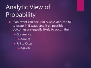
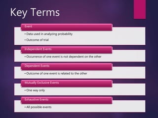
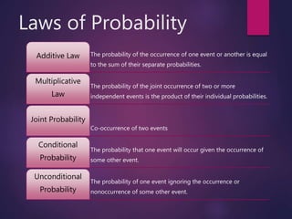
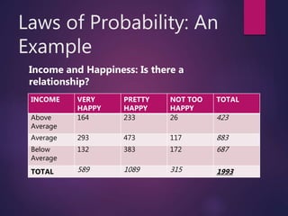
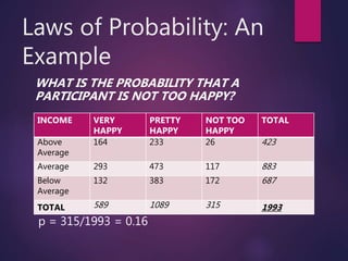
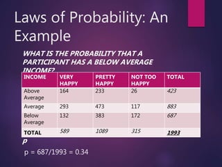
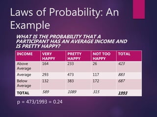
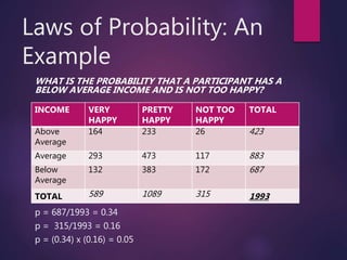
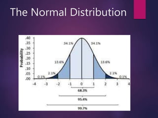
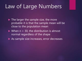
Probability
&
Probability
Distribution
Analytic View of
Probability
 If an event can occur in A ways and can fail
to occur in B ways, and if all possible
outcomes are equally likely to occur, then:
 Occurrence:
 A/(A+B)
 Fail to Occur:
 B/(A+B)
Frequentist View of
Probability
 Probability is defined in terms of one’s past
performance
 Uses sampling with replacement/independent
random sampling
Subjective Probability
 An individuals subjective belief in the
likelihood of occurrence
Key Terms
• Data used in analyzing probability
• Outcome of trial
Event
• Occurrence of one event is not dependent on the other
Independent Events
• Outcome of one event is related to the other
Dependent Events
• One way only
Mutually Exclusive Events
• All possible events
Exhaustive Events
Laws of Probability
The probability of the occurrence of one event or another is equal
to the sum of their separate probabilities.
Additive Law
The probability of the joint occurrence of two or more
independent events is the product of their individual probabilities.
Multiplicative
Law
Co-occurrence of two events
Joint Probability
The probability that one event will occur given the occurrence of
some other event.
Conditional
Probability
The probability of one event ignoring the occurrence or
nonoccurrence of some other event.
Unconditional
Probability
Laws of Probability: An
Example
Income and Happiness: Is there a
relationship?
INCOME VERY
HAPPY
PRETTY
HAPPY
NOT TOO
HAPPY
TOTAL
Above
Average
164 233 26 423
Average 293 473 117 883
Below
Average
132 383 172 687
TOTAL 589 1089 315 1993
Laws of Probability: An
Example
WHAT IS THE PROBABILITY THAT A
PARTICIPANT IS NOT TOO HAPPY?
p
p = 315/1993 = 0.16
INCOME VERY
HAPPY
PRETTY
HAPPY
NOT TOO
HAPPY
TOTAL
Above
Average
164 233 26 423
Average 293 473 117 883
Below
Average
132 383 172 687
TOTAL 589 1089 315 1993
Laws of Probability: An
Example
WHAT IS THE PROBABILITY THAT A
PARTICIPANT HAS A BELOW AVERAGE
INCOME?
p
p = 687/1993 = 0.34
INCOME VERY
HAPPY
PRETTY
HAPPY
NOT TOO
HAPPY
TOTAL
Above
Average
164 233 26 423
Average 293 473 117 883
Below
Average
132 383 172 687
TOTAL 589 1089 315 1993
Laws of Probability: An
Example
WHAT IS THE PROBABILITY THAT A
PARTICIPANT HAS AN AVERAGE INCOME AND
IS PRETTY HAPPY?
p = 473/1993 = 0.24
INCOME VERY
HAPPY
PRETTY
HAPPY
NOT TOO
HAPPY
TOTAL
Above
Average
164 233 26 423
Average 293 473 117 883
Below
Average
132 383 172 687
TOTAL 589 1089 315 1993
Laws of Probability: An
Example
WHAT IS THE PROBABILITY THAT A
PARTICIPANT HAS A BELOW AVERAGE
INCOME GIVEN THAT HE/SHE IS VERY HAPPY?
p = 132/687 = 0.19
INCOME VERY
HAPPY
PRETTY
HAPPY
NOT TOO
HAPPY
TOTAL
Above
Average
164 233 26 423
Average 293 473 117 883
Below
Average
132 383 172 687
TOTAL 589 1089 315 1993
Laws of Probability: An
Example
WHAT IS THE PROBABILITY THAT A PARTICIPANT HAS A
BELOW AVERAGE INCOME AND IS NOT TOO HAPPY?
p = 687/1993 = 0.34
p = 315/1993 = 0.16
p = (0.34) x (0.16) = 0.05
INCOME VERY
HAPPY
PRETTY
HAPPY
NOT TOO
HAPPY
TOTAL
Above
Average
164 233 26 423
Average 293 473 117 883
Below
Average
132 383 172 687
TOTAL 589 1089 315 1993
The Normal Distribution
 Symmetrical
 Bell-shaped
 Mean, Median, and Mode are equal to one
another
The Normal Distribution
 The use of z-scores can help determine the
probability
 Can describe the proportions of area
contained in each section of the distribution
The Normal Distribution
 The use of z-scores can help determine the
probability
 Can describe the proportions of area
contained in each section of the distribution
z-scores
 Helps identify the exact location of a score
in a distribution
 To make raw scores meaningful, they are
transformed into new values
 Standardizes the entire distribution
z-scores
𝑧 =
𝑥 − 𝑥
𝜎
𝑥 = 𝜇 + 𝑧𝜎
Example 1
SAT scores for a normal distribution with
mean of 500 and a standard deviation of 100.
What SAT score separates the top 10% of the
distribution from the test?
Solution 1
X = mean + (z) (sd)
X = 500 + (z) (100)
X = 500 + (1.28) (100)
X = 500 + 128
X = 628
Example 2
IQ test scores are standardized to produce a
normal distribution with a mean of 100 and a
standard deviation of 15. Find the proportion
of the population in each of the following IQ
categories:
Genius or near genius: IQ over 140
Very superior: IQ 120-140
Average: IQ 90-109
Solution 2
Genius or near genius:
z = 140-100/15
z = 2.67
p = 0.0038 or 3.8%
Very Superior:
z = 120-100/15 = 1.33
z = 140-100/15 = 2.67
p (120 < X < 140) = 0. 0918 – 0.0038
p = 0.0880 or 8.8%
Average:
z = 90-100/15 = -0.67
z = 109-100/15 = 0.60
p = (90 < X < 109) = 0.2486 + 0.2257
p = 0.4744 or 47.44%
Sampling Error
 Discrepancy between a sample statistic and
its corresponding population parameter
 If the population is normal, you should be
able to determine the probability of
obtaining any individual score
Sampling Distribution
 Distribution of statistics obtained by
selecting all the possible samples of a
specific size from a population
Distribution of Sample
Means
 Collection of sample means for all possible
random samples of a particular size that can
be obtained from a population
 Characteristics:
 Piles up around population mean
 Forms a normal distribution
 The larger the sample size, the closer to the
population mean
Central Limit Theorem
 For any population with mean and standard
deviation, the distribution of sample means
for sample size will have a mean and a
standard deviation ( 𝜎 𝑛) that will
approach a normal distribution as the
sample approaches infinity.
Central Limit Theorem
 Expected Value of M
 The mean of the distribution of sample
means is equal to the mean of the
population of scores
 Standard Error of M
 Provides a measure on how much distance is
expected between sample mean and population
mean
Law of Large Numbers
 The larger the sample size, the more
probable it is that the sample mean will be
close to the population mean
 When n > 30, the distribution is almost
normal regardless of the shape
 As sample size increases, error decreases

Psych stats Probability and Probability Distribution

  • 1.
  • 2.
    Analytic View of Probability If an event can occur in A ways and can fail to occur in B ways, and if all possible outcomes are equally likely to occur, then:  Occurrence:  A/(A+B)  Fail to Occur:  B/(A+B)
  • 3.
    Frequentist View of Probability Probability is defined in terms of one’s past performance  Uses sampling with replacement/independent random sampling
  • 4.
    Subjective Probability  Anindividuals subjective belief in the likelihood of occurrence
  • 5.
    Key Terms • Dataused in analyzing probability • Outcome of trial Event • Occurrence of one event is not dependent on the other Independent Events • Outcome of one event is related to the other Dependent Events • One way only Mutually Exclusive Events • All possible events Exhaustive Events
  • 6.
    Laws of Probability Theprobability of the occurrence of one event or another is equal to the sum of their separate probabilities. Additive Law The probability of the joint occurrence of two or more independent events is the product of their individual probabilities. Multiplicative Law Co-occurrence of two events Joint Probability The probability that one event will occur given the occurrence of some other event. Conditional Probability The probability of one event ignoring the occurrence or nonoccurrence of some other event. Unconditional Probability
  • 7.
    Laws of Probability:An Example Income and Happiness: Is there a relationship? INCOME VERY HAPPY PRETTY HAPPY NOT TOO HAPPY TOTAL Above Average 164 233 26 423 Average 293 473 117 883 Below Average 132 383 172 687 TOTAL 589 1089 315 1993
  • 8.
    Laws of Probability:An Example WHAT IS THE PROBABILITY THAT A PARTICIPANT IS NOT TOO HAPPY? p p = 315/1993 = 0.16 INCOME VERY HAPPY PRETTY HAPPY NOT TOO HAPPY TOTAL Above Average 164 233 26 423 Average 293 473 117 883 Below Average 132 383 172 687 TOTAL 589 1089 315 1993
  • 9.
    Laws of Probability:An Example WHAT IS THE PROBABILITY THAT A PARTICIPANT HAS A BELOW AVERAGE INCOME? p p = 687/1993 = 0.34 INCOME VERY HAPPY PRETTY HAPPY NOT TOO HAPPY TOTAL Above Average 164 233 26 423 Average 293 473 117 883 Below Average 132 383 172 687 TOTAL 589 1089 315 1993
  • 10.
    Laws of Probability:An Example WHAT IS THE PROBABILITY THAT A PARTICIPANT HAS AN AVERAGE INCOME AND IS PRETTY HAPPY? p = 473/1993 = 0.24 INCOME VERY HAPPY PRETTY HAPPY NOT TOO HAPPY TOTAL Above Average 164 233 26 423 Average 293 473 117 883 Below Average 132 383 172 687 TOTAL 589 1089 315 1993
  • 11.
    Laws of Probability:An Example WHAT IS THE PROBABILITY THAT A PARTICIPANT HAS A BELOW AVERAGE INCOME GIVEN THAT HE/SHE IS VERY HAPPY? p = 132/687 = 0.19 INCOME VERY HAPPY PRETTY HAPPY NOT TOO HAPPY TOTAL Above Average 164 233 26 423 Average 293 473 117 883 Below Average 132 383 172 687 TOTAL 589 1089 315 1993
  • 12.
    Laws of Probability:An Example WHAT IS THE PROBABILITY THAT A PARTICIPANT HAS A BELOW AVERAGE INCOME AND IS NOT TOO HAPPY? p = 687/1993 = 0.34 p = 315/1993 = 0.16 p = (0.34) x (0.16) = 0.05 INCOME VERY HAPPY PRETTY HAPPY NOT TOO HAPPY TOTAL Above Average 164 233 26 423 Average 293 473 117 883 Below Average 132 383 172 687 TOTAL 589 1089 315 1993
  • 13.
    The Normal Distribution Symmetrical  Bell-shaped  Mean, Median, and Mode are equal to one another
  • 14.
  • 15.
    The Normal Distribution The use of z-scores can help determine the probability  Can describe the proportions of area contained in each section of the distribution
  • 16.
    The Normal Distribution The use of z-scores can help determine the probability  Can describe the proportions of area contained in each section of the distribution
  • 17.
    z-scores  Helps identifythe exact location of a score in a distribution  To make raw scores meaningful, they are transformed into new values  Standardizes the entire distribution
  • 18.
    z-scores 𝑧 = 𝑥 −𝑥 𝜎 𝑥 = 𝜇 + 𝑧𝜎
  • 19.
    Example 1 SAT scoresfor a normal distribution with mean of 500 and a standard deviation of 100. What SAT score separates the top 10% of the distribution from the test?
  • 20.
    Solution 1 X =mean + (z) (sd) X = 500 + (z) (100) X = 500 + (1.28) (100) X = 500 + 128 X = 628
  • 21.
    Example 2 IQ testscores are standardized to produce a normal distribution with a mean of 100 and a standard deviation of 15. Find the proportion of the population in each of the following IQ categories: Genius or near genius: IQ over 140 Very superior: IQ 120-140 Average: IQ 90-109
  • 22.
    Solution 2 Genius ornear genius: z = 140-100/15 z = 2.67 p = 0.0038 or 3.8% Very Superior: z = 120-100/15 = 1.33 z = 140-100/15 = 2.67 p (120 < X < 140) = 0. 0918 – 0.0038 p = 0.0880 or 8.8% Average: z = 90-100/15 = -0.67 z = 109-100/15 = 0.60 p = (90 < X < 109) = 0.2486 + 0.2257 p = 0.4744 or 47.44%
  • 23.
    Sampling Error  Discrepancybetween a sample statistic and its corresponding population parameter  If the population is normal, you should be able to determine the probability of obtaining any individual score
  • 24.
    Sampling Distribution  Distributionof statistics obtained by selecting all the possible samples of a specific size from a population
  • 25.
    Distribution of Sample Means Collection of sample means for all possible random samples of a particular size that can be obtained from a population  Characteristics:  Piles up around population mean  Forms a normal distribution  The larger the sample size, the closer to the population mean
  • 26.
    Central Limit Theorem For any population with mean and standard deviation, the distribution of sample means for sample size will have a mean and a standard deviation ( 𝜎 𝑛) that will approach a normal distribution as the sample approaches infinity.
  • 27.
    Central Limit Theorem Expected Value of M  The mean of the distribution of sample means is equal to the mean of the population of scores  Standard Error of M  Provides a measure on how much distance is expected between sample mean and population mean
  • 28.
    Law of LargeNumbers  The larger the sample size, the more probable it is that the sample mean will be close to the population mean  When n > 30, the distribution is almost normal regardless of the shape  As sample size increases, error decreases