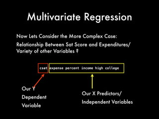
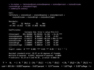
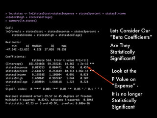
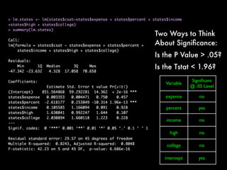
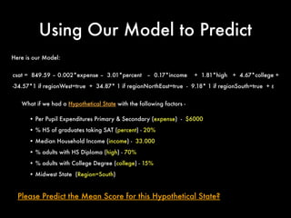
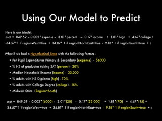
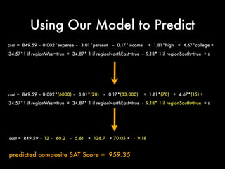
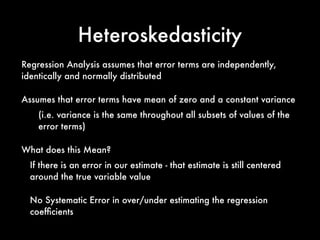
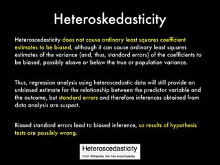
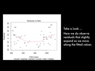
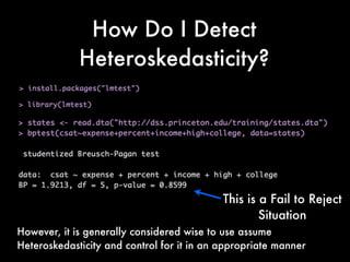
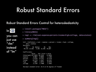
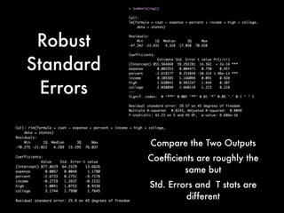
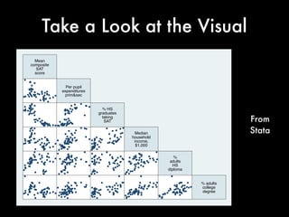
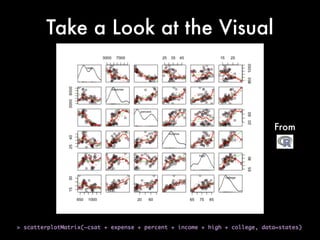
Quantitative
Methods
for
Lawyers Class #20
Regression Analysis
Part 3
@ computational
computationallegalstudies.com
professor daniel martin katz danielmartinkatz.com
lexpredict.com slideshare.net/DanielKatz
Multiple
Regression
Just a Reminder...
Keep This Visual Image
in Your Mind
Estimate a lawyer’s rate:
Real Rate Report™ Regression model
From the CT TyMetrix/Corporate Executive Board 2012
Real Rate Report©
$15
1
$16
1
$34
per 10 years$95 +$99
(Finance)
-$15
(Litigation)
n = 15,353 Lawyers
Tier 1
Market Experience
Partner
Status
Practice
Area
Base
+ + +/-
Source: 2012 Real Rate Report™
32
$15
Per
100 Lawyers
Law
Firm
Size+ +
$161
$151
$15
per 100
lawyers $95
$34
per 10
years
-$15
(Litigation)
+$99
(Finance)
Y = βo +/- β1 ( X1 ) +/- β2 ( X2 ) +/- β3 ( X3 ) +/- β4 ( X3 ) +/- β5 ( X3 ) + ε
Y = $151 + $15 ( ) + 161 ( ) + 95 ( ) + 34 ( ) +/- β5 ( ) + ε
Per
100
Lawyers
If Tier 1
Market
is True
Partner
Status
is True
Per
10
Years
Practice
Area
From The Last Time...
Now Lets Consider the More Complex Case:
Relationship Between Sat Score and Expenditures/
Variety of other Variables ?
Our Y
Dependent
Variable
Our X Predictors/
Independent Variables
Multivariate Regression
Y = B0 + ( B1 * (X1) ) – ( B2 * (X2) ) + ( B3 * (X3) ) + ( B4 * (X4)) + ( B5 * (X5) ) + ε
csat = 851.56 + 0.003*expense – 2.62*percent + 0.11*income + 1.63*high + 2.03*college + ε
Lets Consider Our
“Beta Coefficients”
Are They
Statistically
Significant?
Look at the
P Value on
“Expense” -
It is no longer
Statistically
Significant
Two Ways to Think
About Significance:
Is the P Value > .05?
Is the Tstat < 1.96?
Variable
Significant
@ .05 Level
expense no
percent yes
income no
high no
college no
intercept yes
Using Our Model to Predict
What if we had a Hypothetical State with the following factors -
• Per Pupil Expenditures Primary & Secondary (expense) - $6000
• % HS of graduates taking SAT (percent) - 20%
• Median Household Income (income) - 33.000
• % adults with HS Diploma (high) - 70%
• % adults with College Degree (college) - 15%
• Midwest State (Region=South)
Please Predict the Mean Score for this Hypothetical State?
Here is our Model:
csat = 849.59 – 0.002*expense – 3.01*percent – 0.17*income + 1.81*high + 4.67*college +
-34.57*1 if regionWest=true + 34.87* 1 if regionNorthEast=true - 9.18* 1 if regionSouth=true + ε
Using Our Model to Predict
What if we had a Hypothetical State with the following factors -
• Per Pupil Expenditures Primary & Secondary (expense) - $6000
• % HS of graduates taking SAT (percent) - 20%
• Median Household Income (income) - 33.000
• % adults with HS Diploma (high) - 70%
• % adults with College Degree (college) - 15%
• Midwest State (Region=South)
Here is our Model:
csat = 849.59 – 0.002*expense – 3.01*percent – 0.17*income + 1.81*high + 4.67*college +
-34.57*1 if regionWest=true + 34.87* 1 if regionNorthEast=true - 9.18* 1 if regionSouth=true + ε
csat = 849.59 – 0.002*(6000) – 3.01*(20) – 0.17*(33.000) + 1.81*(70) + 4.67*(15) +
-34.57*1 if regionWest=true + 34.87* 1 if regionNorthEast=true - 9.18* 1 if regionSouth=true + ε
Using Our Model to Predict
csat = 849.59 – 0.002*(6000) – 3.01*(20) – 0.17*(33.000) + 1.81*(70) + 4.67*(15) +
-34.57*1 if regionWest=true + 34.87* 1 if regionNorthEast=true - 9.18* 1 if regionSouth=true + ε
csat = 849.59 – 0.002*expense – 3.01*percent – 0.17*income + 1.81*high + 4.67*college +
-34.57*1 if regionWest=true + 34.87* 1 if regionNorthEast=true - 9.18* 1 if regionSouth=true + ε
csat = 849.59 – 12 – 60.2 – 5.61 + 126.7 + 70.05 + - 9.18
predicted composite SAT Score = 959.35
Violation of
Regression
Assumptions
Heteroskedasticity
Regression Analysis assumes that error terms are independently,
identically and normally distributed
Assumes that error terms have mean of zero and a constant variance
(i.e. variance is the same throughout all subsets of values of the
error terms)
What does this Mean?
If there is an error in our estimate - that estimate is still centered
around the true variable value
No Systematic Error in over/under estimating the regression
coefficients
Heteroskedasticity
Heteroscedasticity does not cause ordinary least squares coefficient
estimates to be biased, although it can cause ordinary least squares
estimates of the variance (and, thus, standard errors) of the coefficients to
be biased, possibly above or below the true or population variance.
Thus, regression analysis using heteroscedastic data will still provide an
unbiased estimate for the relationship between the predictor variable and
the outcome, but standard errors and therefore inferences obtained from
data analysis are suspect.
Biased standard errors lead to biased inference, so results of hypothesis
tests are possibly wrong.
Heteroskedasticity
HeteroskedasticHomoskedastic
How Do I Detect
Heteroskedasticity?
Visual (Ocular) Method is a good starting point (although you
should probably also check with a more formal approach)
However, lets just start here:
(1) Run the Regression
(2) Plot the Residuals against the fitted values
(3) Review the Resulting Plot -
When plotting residuals vs. predicted values (aka Yhat) we
should not observe any pattern if the variance in the
residuals is homoskedastic
(0) Load the Data
(1) Run the Regression
(2) Plot the Residuals against the fitted values
(3) Review the Resulting Plot -
When plotting residuals vs. predicted values
(aka Yhat) we should not observe any pattern
if the variance in the residuals is
homoskedastic
Take a Look ...
Here we do observe
residuals that slightly
expand as we move
along the fitted values
How Do I Detect
Heteroskedasticity?
There is a More Formal Approach ...
the Breusch-Pagan test
Test the Null Hypothesis of Constant Variance
(1) Run the Regression
(2) Execute the Breusch-Pagan test
How Do I Detect
Heteroskedasticity?
However, it is generally considered wise to use assume
Heteroskedasticity and control for it in an appropriate manner
This is a Fail to Reject
Situation
Robust
Standard
Errors
Robust Standard Errors
Robust Standard Errors Control for heteroskedasticity
In R
you can
just use
“rlm”
instead
of “lm”
Robust
Standard
Errors
Compare the Two Outputs
Coefficients are roughly the
same but
Std. Errors and T stats are
different
Multicollinearity
Multicollinearity
statistical phenomenon in which two or more predictor variables in
a multiple regression model are highly correlated.
In this situation the coefficient estimates may change erratically in
response to small changes in the model or the data.
Multicollinearity does not reduce the predictive power or reliability
of the model as a whole, at least within the sample data
themselves; it only affects calculations regarding individual
predictors.
Take a Look at the Visual
Mean
composite
SAT
score
Per pupil
expenditures
prim&sec
% HS
graduates
taking
SAT
Median
household
income,
$1,000
%
adults
HS
diploma
% adults
college
degree
From
Stata
Take a Look at the Visual
From
R
Take a Look at the Visual
Mean
composite
SAT
score
Per pupil
expenditures
prim&sec
% HS
graduates
taking
SAT
Median
household
income,
$1,000
%
adults
HS
diploma
% adults
college
degree
http://cran.r-project.org/web/packages/car/car.pdf
How Do I Detect
Multicollinearity?
(1) Run the Regression
(2) Obtain and then Examine the Variance Inflation Factor (“VIF”)
A vif > 10 or a 1/vif < 0.10 is an issue
Here we look to be okay
Daniel Martin Katz
@ computational
computationallegalstudies.com
lexpredict.com
danielmartinkatz.com
illinois tech - chicago kent college of law@

Quantitative Methods for Lawyers - Class #20 - Regression Analysis - Part 3

  • 1.
    Quantitative Methods for Lawyers Class #20 RegressionAnalysis Part 3 @ computational computationallegalstudies.com professor daniel martin katz danielmartinkatz.com lexpredict.com slideshare.net/DanielKatz
  • 2.
  • 3.
  • 4.
    Keep This VisualImage in Your Mind
  • 5.
    Estimate a lawyer’srate: Real Rate Report™ Regression model From the CT TyMetrix/Corporate Executive Board 2012 Real Rate Report© $15 1 $16 1 $34 per 10 years$95 +$99 (Finance) -$15 (Litigation) n = 15,353 Lawyers Tier 1 Market Experience Partner Status Practice Area Base + + +/- Source: 2012 Real Rate Report™ 32 $15 Per 100 Lawyers Law Firm Size+ + $161 $151 $15 per 100 lawyers $95 $34 per 10 years -$15 (Litigation) +$99 (Finance)
  • 6.
    Y = βo+/- β1 ( X1 ) +/- β2 ( X2 ) +/- β3 ( X3 ) +/- β4 ( X3 ) +/- β5 ( X3 ) + ε Y = $151 + $15 ( ) + 161 ( ) + 95 ( ) + 34 ( ) +/- β5 ( ) + ε Per 100 Lawyers If Tier 1 Market is True Partner Status is True Per 10 Years Practice Area
  • 7.
  • 8.
    Now Lets Considerthe More Complex Case: Relationship Between Sat Score and Expenditures/ Variety of other Variables ? Our Y Dependent Variable Our X Predictors/ Independent Variables Multivariate Regression
  • 9.
    Y = B0+ ( B1 * (X1) ) – ( B2 * (X2) ) + ( B3 * (X3) ) + ( B4 * (X4)) + ( B5 * (X5) ) + ε csat = 851.56 + 0.003*expense – 2.62*percent + 0.11*income + 1.63*high + 2.03*college + ε
  • 10.
    Lets Consider Our “BetaCoefficients” Are They Statistically Significant? Look at the P Value on “Expense” - It is no longer Statistically Significant
  • 11.
    Two Ways toThink About Significance: Is the P Value > .05? Is the Tstat < 1.96? Variable Significant @ .05 Level expense no percent yes income no high no college no intercept yes
  • 12.
    Using Our Modelto Predict
  • 13.
    Using Our Modelto Predict What if we had a Hypothetical State with the following factors - • Per Pupil Expenditures Primary & Secondary (expense) - $6000 • % HS of graduates taking SAT (percent) - 20% • Median Household Income (income) - 33.000 • % adults with HS Diploma (high) - 70% • % adults with College Degree (college) - 15% • Midwest State (Region=South) Please Predict the Mean Score for this Hypothetical State? Here is our Model: csat = 849.59 – 0.002*expense – 3.01*percent – 0.17*income + 1.81*high + 4.67*college + -34.57*1 if regionWest=true + 34.87* 1 if regionNorthEast=true - 9.18* 1 if regionSouth=true + ε
  • 14.
    Using Our Modelto Predict What if we had a Hypothetical State with the following factors - • Per Pupil Expenditures Primary & Secondary (expense) - $6000 • % HS of graduates taking SAT (percent) - 20% • Median Household Income (income) - 33.000 • % adults with HS Diploma (high) - 70% • % adults with College Degree (college) - 15% • Midwest State (Region=South) Here is our Model: csat = 849.59 – 0.002*expense – 3.01*percent – 0.17*income + 1.81*high + 4.67*college + -34.57*1 if regionWest=true + 34.87* 1 if regionNorthEast=true - 9.18* 1 if regionSouth=true + ε csat = 849.59 – 0.002*(6000) – 3.01*(20) – 0.17*(33.000) + 1.81*(70) + 4.67*(15) + -34.57*1 if regionWest=true + 34.87* 1 if regionNorthEast=true - 9.18* 1 if regionSouth=true + ε
  • 15.
    Using Our Modelto Predict csat = 849.59 – 0.002*(6000) – 3.01*(20) – 0.17*(33.000) + 1.81*(70) + 4.67*(15) + -34.57*1 if regionWest=true + 34.87* 1 if regionNorthEast=true - 9.18* 1 if regionSouth=true + ε csat = 849.59 – 0.002*expense – 3.01*percent – 0.17*income + 1.81*high + 4.67*college + -34.57*1 if regionWest=true + 34.87* 1 if regionNorthEast=true - 9.18* 1 if regionSouth=true + ε csat = 849.59 – 12 – 60.2 – 5.61 + 126.7 + 70.05 + - 9.18 predicted composite SAT Score = 959.35
  • 16.
  • 17.
    Heteroskedasticity Regression Analysis assumesthat error terms are independently, identically and normally distributed Assumes that error terms have mean of zero and a constant variance (i.e. variance is the same throughout all subsets of values of the error terms) What does this Mean? If there is an error in our estimate - that estimate is still centered around the true variable value No Systematic Error in over/under estimating the regression coefficients
  • 18.
    Heteroskedasticity Heteroscedasticity does notcause ordinary least squares coefficient estimates to be biased, although it can cause ordinary least squares estimates of the variance (and, thus, standard errors) of the coefficients to be biased, possibly above or below the true or population variance. Thus, regression analysis using heteroscedastic data will still provide an unbiased estimate for the relationship between the predictor variable and the outcome, but standard errors and therefore inferences obtained from data analysis are suspect. Biased standard errors lead to biased inference, so results of hypothesis tests are possibly wrong.
  • 19.
  • 20.
    How Do IDetect Heteroskedasticity? Visual (Ocular) Method is a good starting point (although you should probably also check with a more formal approach) However, lets just start here: (1) Run the Regression (2) Plot the Residuals against the fitted values (3) Review the Resulting Plot - When plotting residuals vs. predicted values (aka Yhat) we should not observe any pattern if the variance in the residuals is homoskedastic
  • 21.
    (0) Load theData (1) Run the Regression
  • 22.
    (1) Run theRegression (2) Plot the Residuals against the fitted values (3) Review the Resulting Plot - When plotting residuals vs. predicted values (aka Yhat) we should not observe any pattern if the variance in the residuals is homoskedastic
  • 23.
    Take a Look... Here we do observe residuals that slightly expand as we move along the fitted values
  • 24.
    How Do IDetect Heteroskedasticity? There is a More Formal Approach ... the Breusch-Pagan test Test the Null Hypothesis of Constant Variance (1) Run the Regression (2) Execute the Breusch-Pagan test
  • 25.
    How Do IDetect Heteroskedasticity? However, it is generally considered wise to use assume Heteroskedasticity and control for it in an appropriate manner This is a Fail to Reject Situation
  • 26.
  • 27.
    Robust Standard Errors RobustStandard Errors Control for heteroskedasticity In R you can just use “rlm” instead of “lm”
  • 28.
    Robust Standard Errors Compare the TwoOutputs Coefficients are roughly the same but Std. Errors and T stats are different
  • 29.
  • 30.
    Multicollinearity statistical phenomenon inwhich two or more predictor variables in a multiple regression model are highly correlated. In this situation the coefficient estimates may change erratically in response to small changes in the model or the data. Multicollinearity does not reduce the predictive power or reliability of the model as a whole, at least within the sample data themselves; it only affects calculations regarding individual predictors.
  • 31.
    Take a Lookat the Visual Mean composite SAT score Per pupil expenditures prim&sec % HS graduates taking SAT Median household income, $1,000 % adults HS diploma % adults college degree From Stata
  • 32.
    Take a Lookat the Visual From R
  • 33.
    Take a Lookat the Visual Mean composite SAT score Per pupil expenditures prim&sec % HS graduates taking SAT Median household income, $1,000 % adults HS diploma % adults college degree
  • 34.
  • 35.
    How Do IDetect Multicollinearity? (1) Run the Regression (2) Obtain and then Examine the Variance Inflation Factor (“VIF”) A vif > 10 or a 1/vif < 0.10 is an issue Here we look to be okay
  • 36.
    Daniel Martin Katz @computational computationallegalstudies.com lexpredict.com danielmartinkatz.com illinois tech - chicago kent college of law@