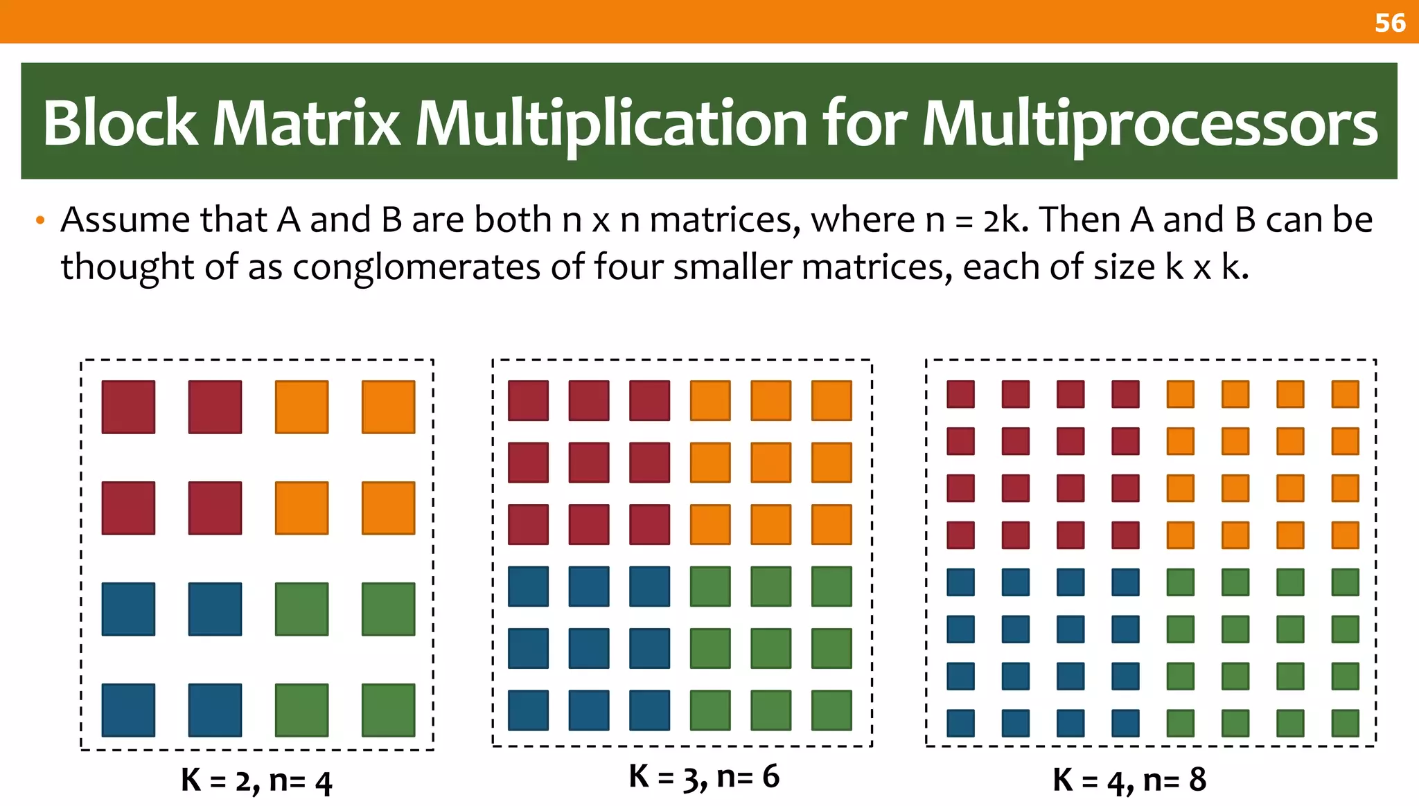
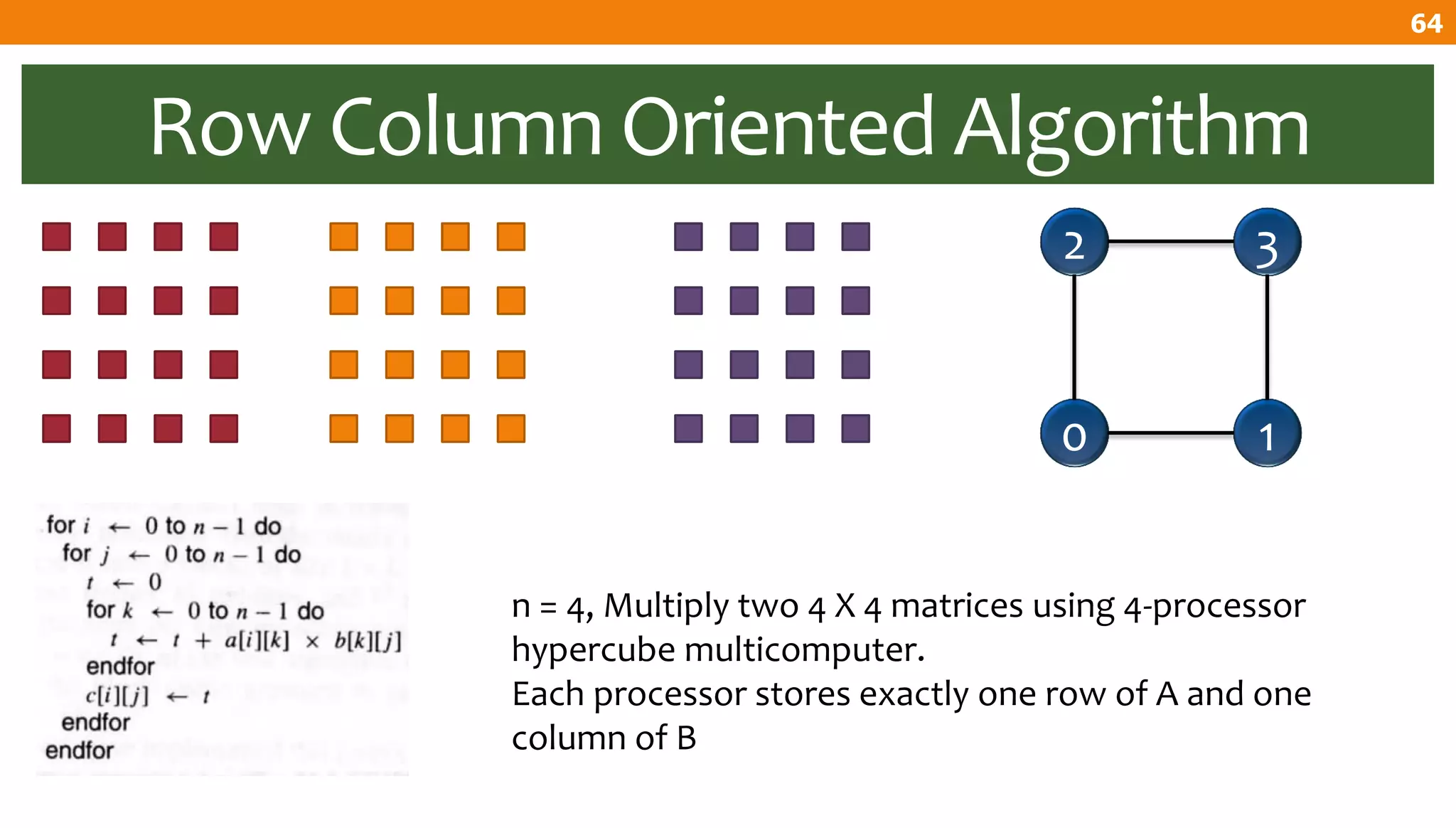
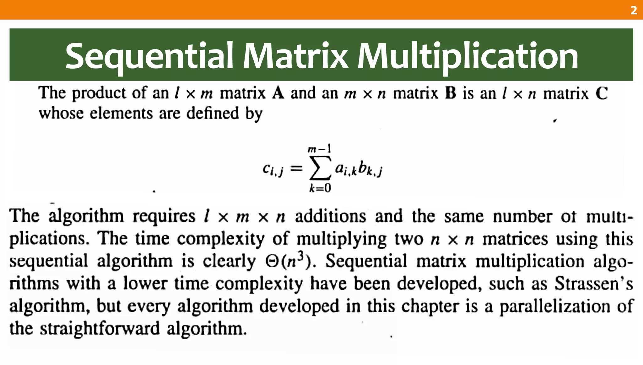
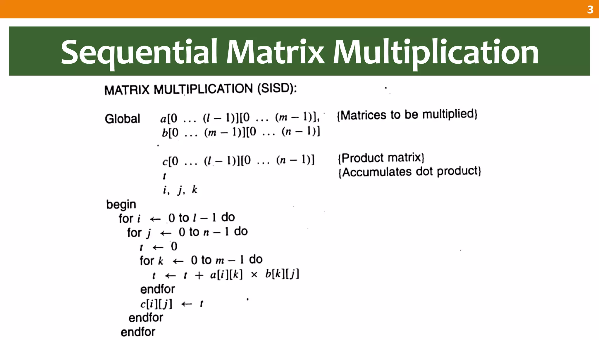
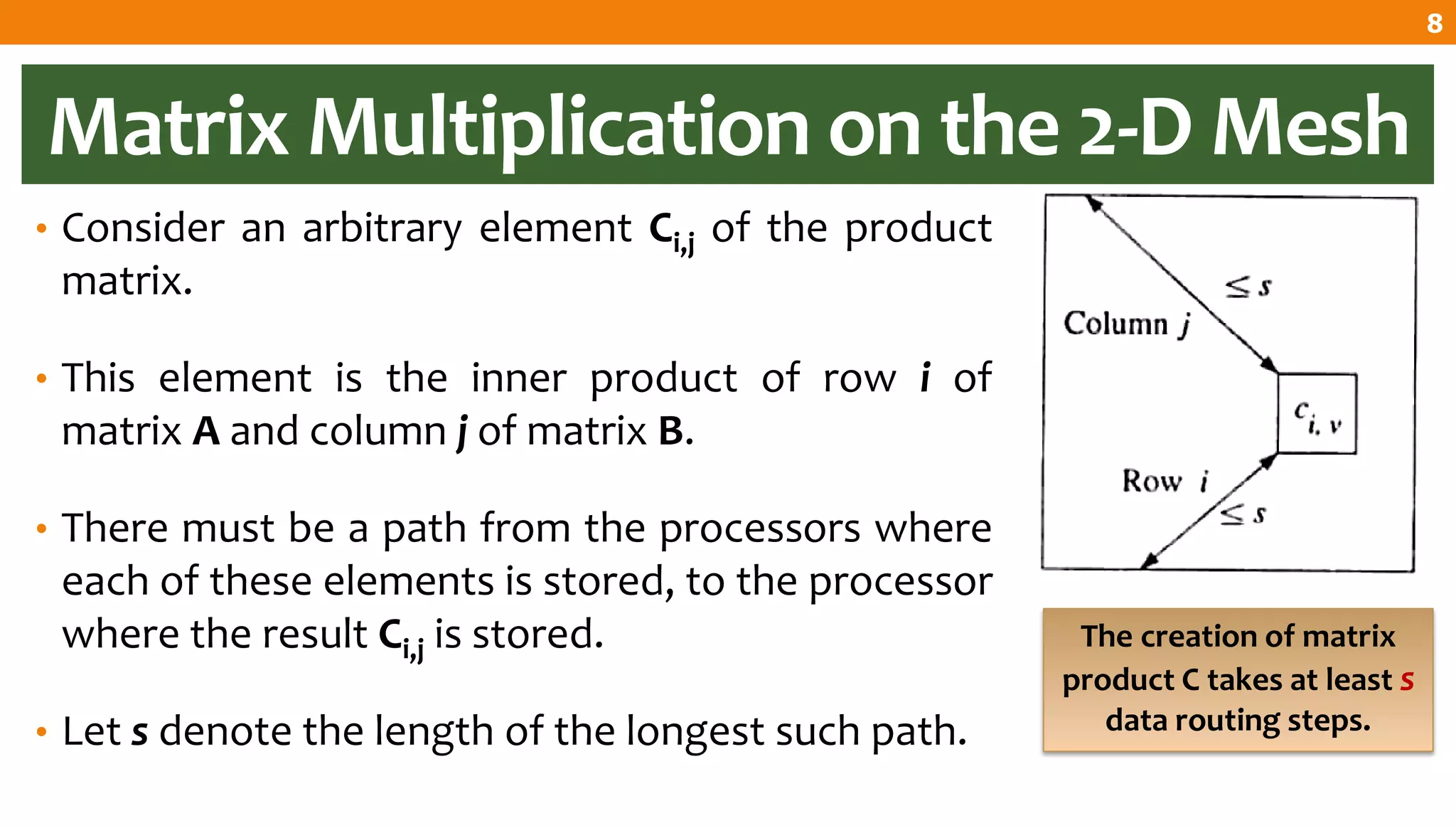
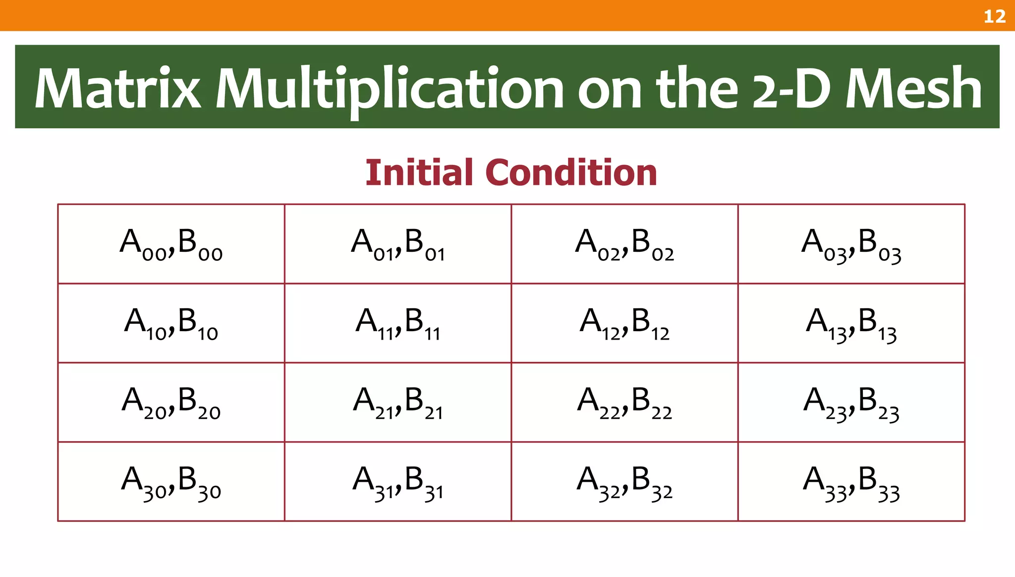
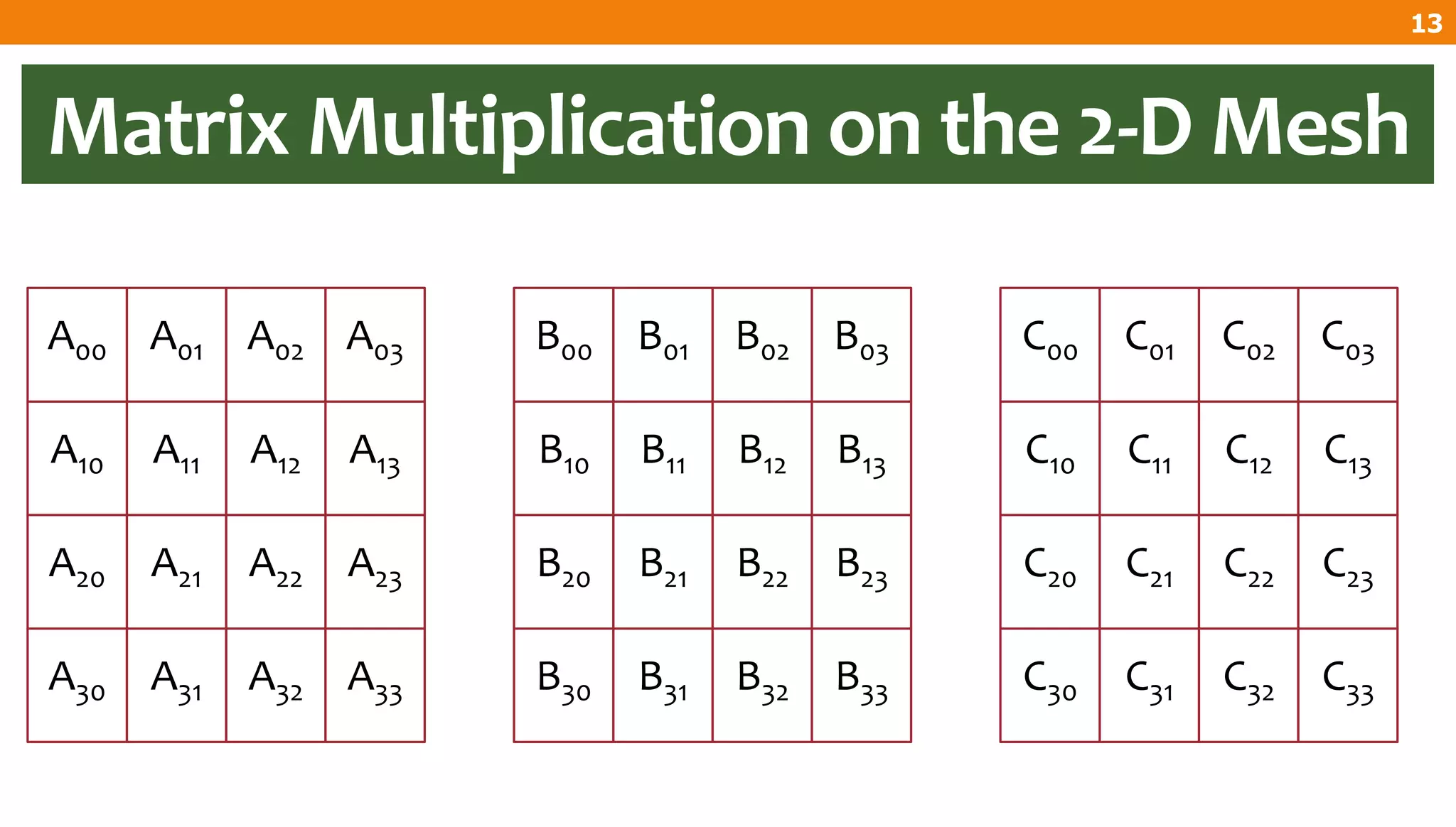
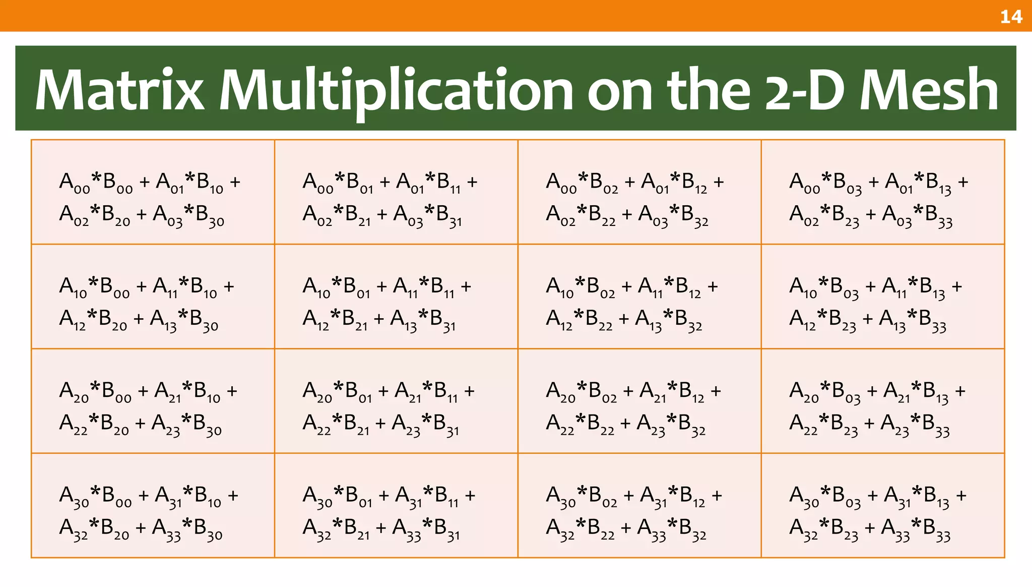
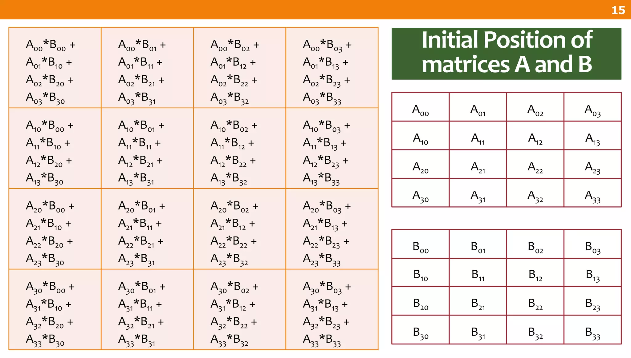
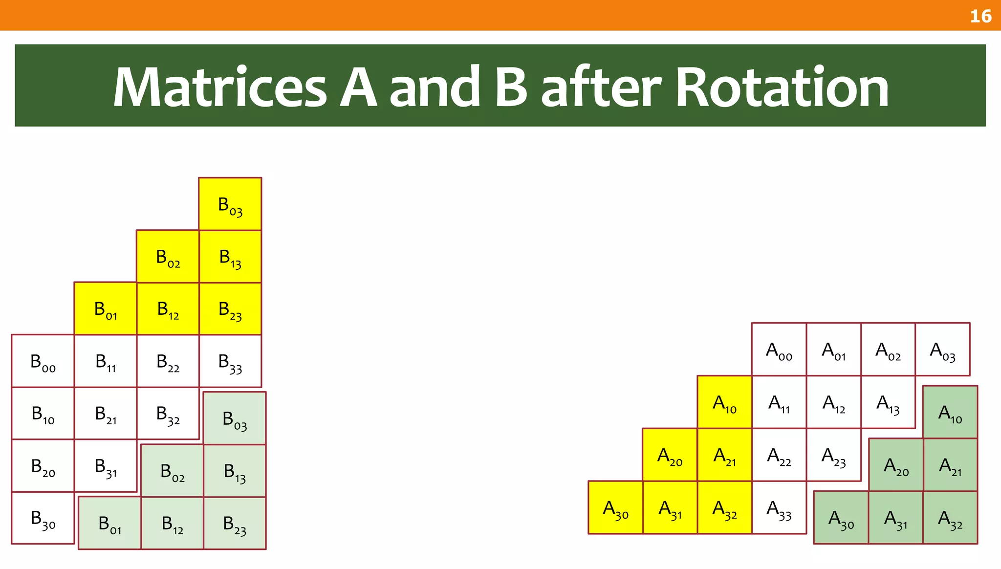
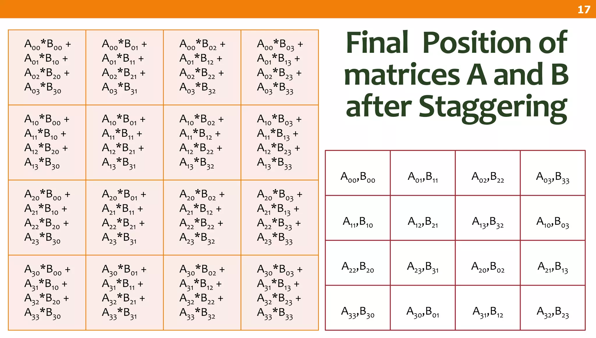
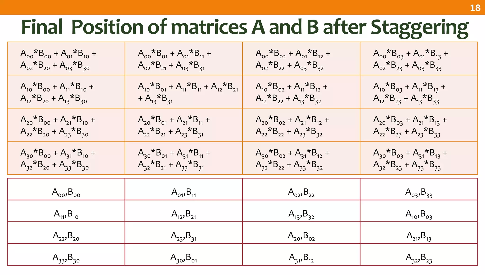
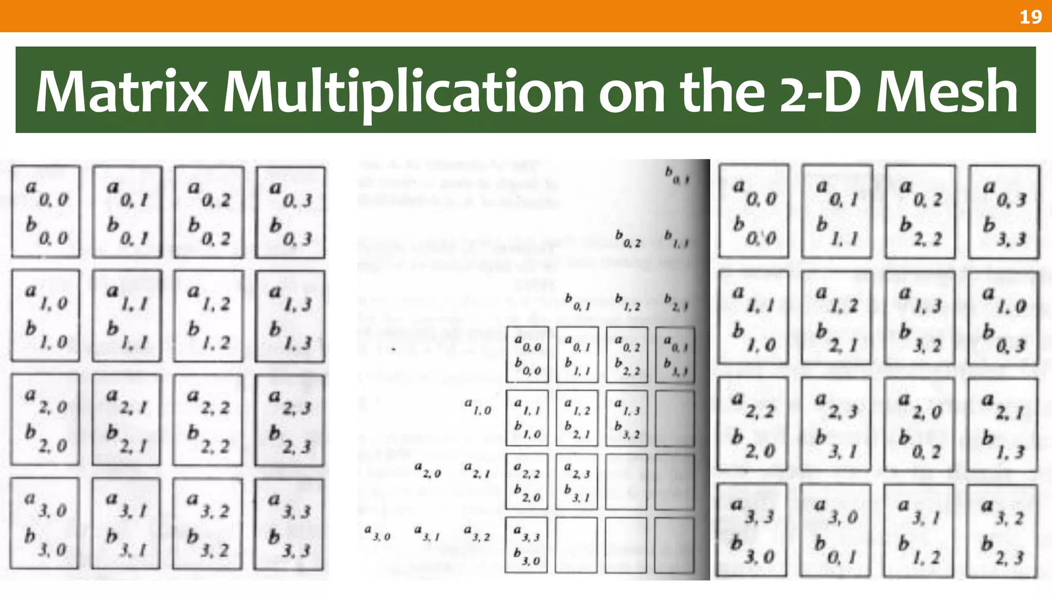
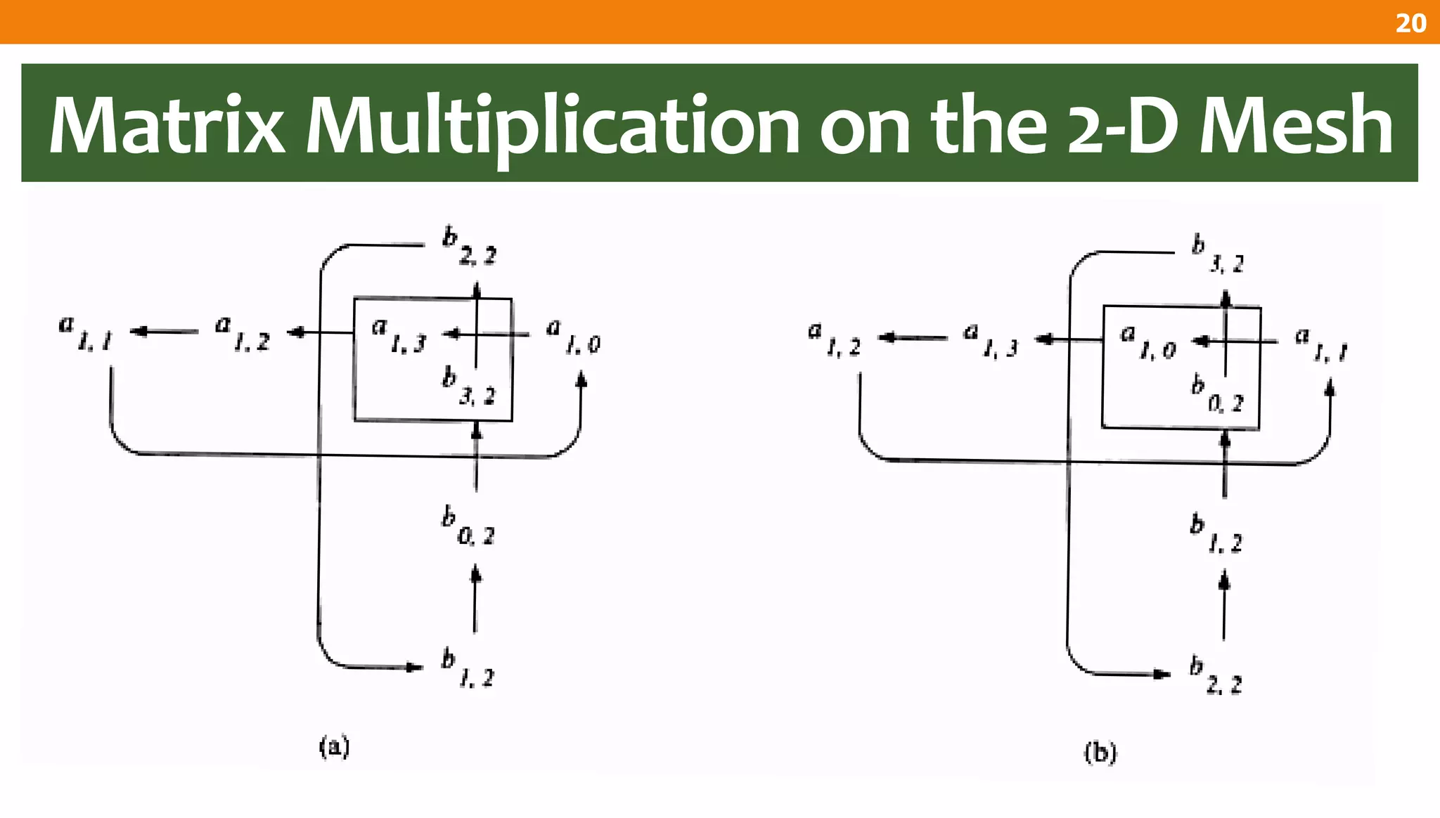
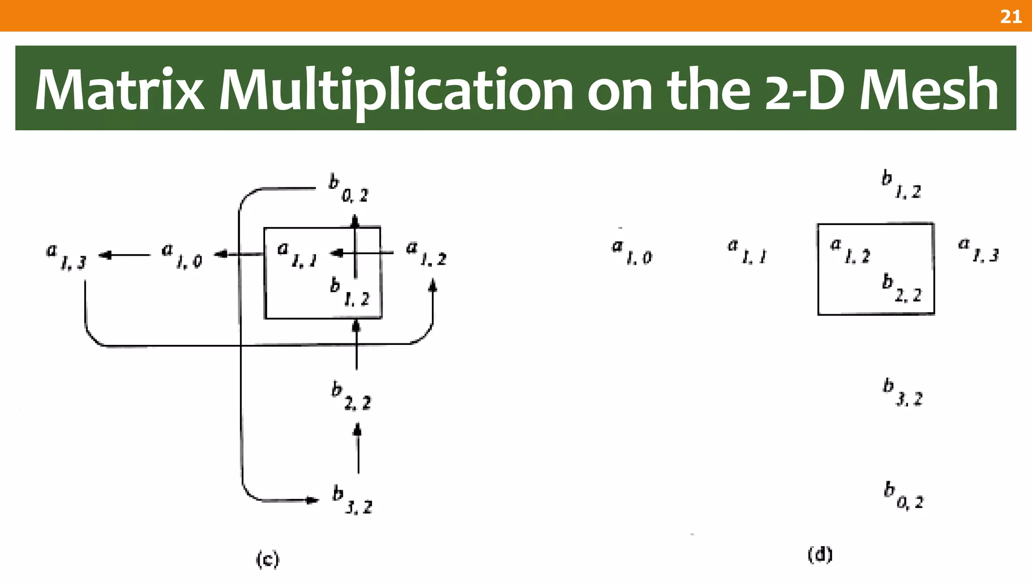
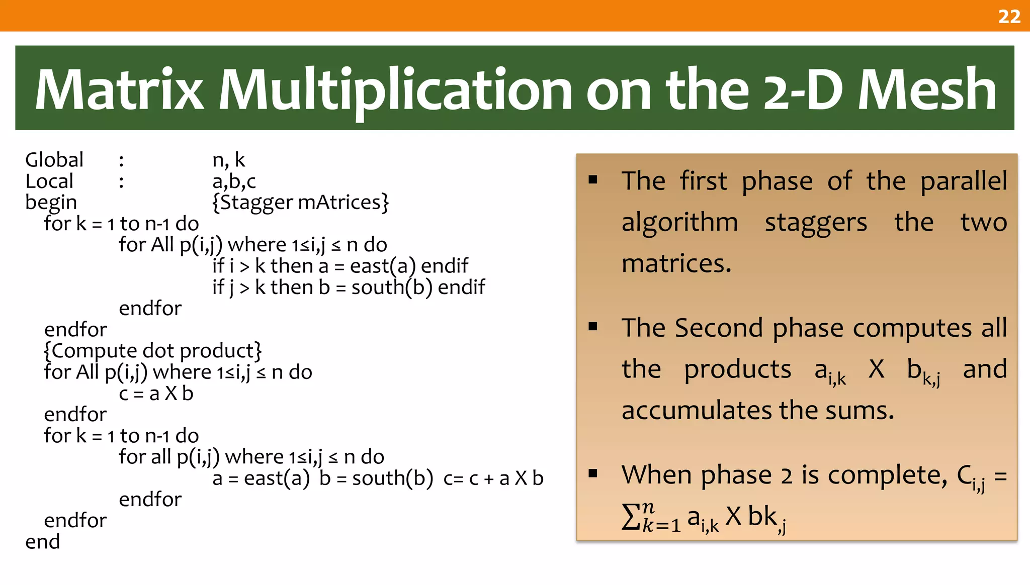
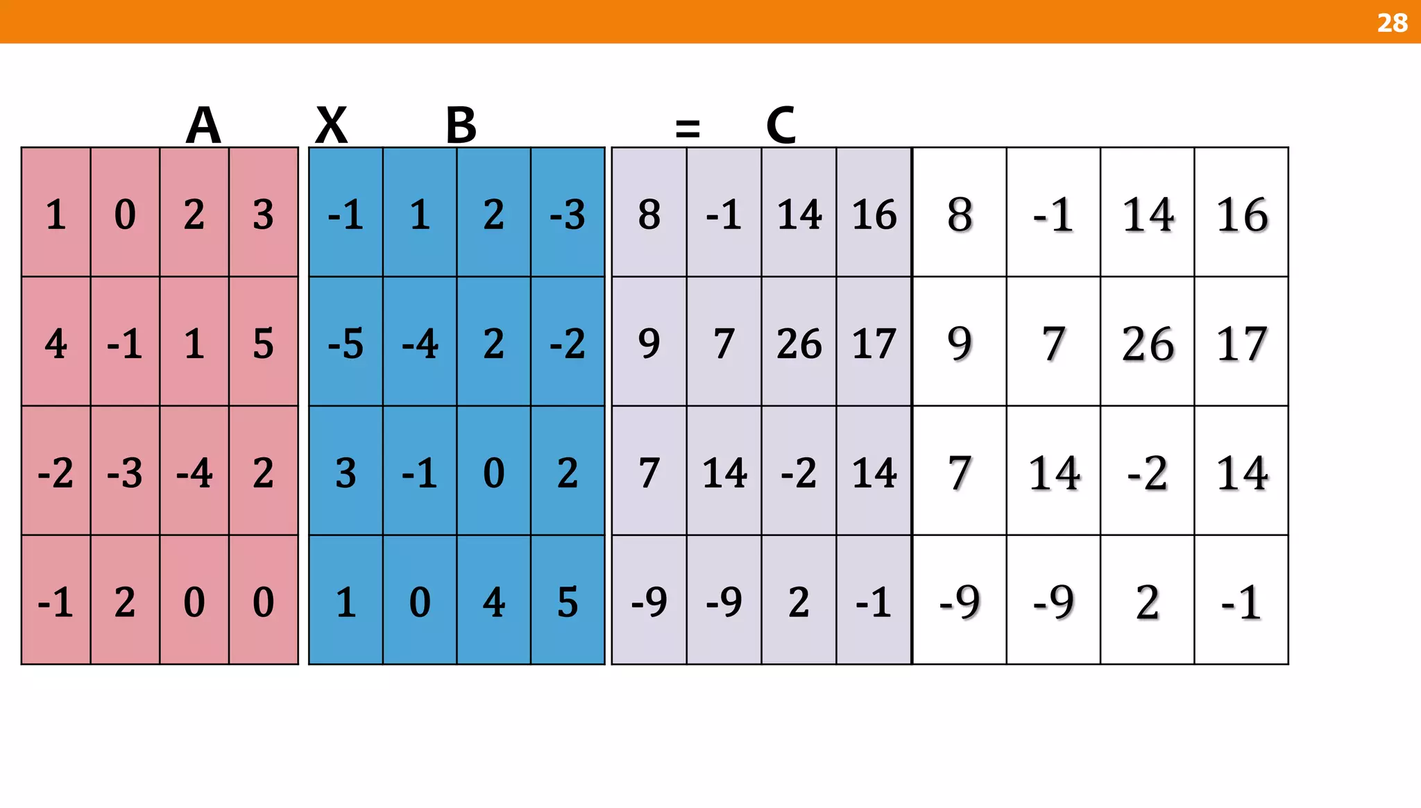
The document describes an algorithm for multiplying two n x n matrices on a 2D mesh parallel computing model. It involves initially staggering the two matrices across the processors in n-1 steps. It then performs a dot product computation of corresponding elements across all processor pairs to calculate the product matrix. This takes advantage of the parallelism available in the mesh to perform the multiplication in O(n) time using n^2 processors.


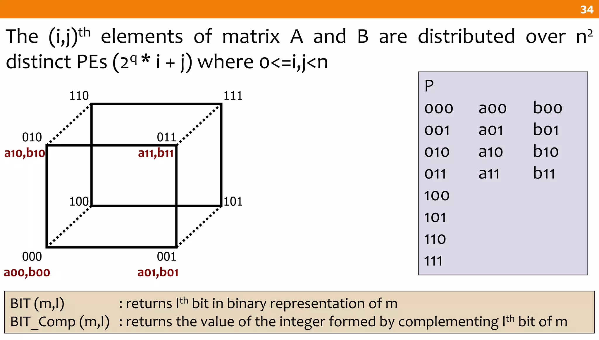
![Matrix Multiplication on Hypercube
K=0
[2*i + j] = ai,j
[2*i + j] = bi,j
K=1
[4 + 2*i + j] = ai,j
[4 + 2*i + j] = bi,j
i, j K=0 K=1
0,0 0 = 000 4 = 100
0,1 1 = 001 5 = 101
1,0 2 = 010 6 = 110
1,1 3 = 011 7 = 111
35](https://image.slidesharecdn.com/chapter-7-201007184022/75/Chapter-7-Matrix-Multiplication-35-2048.jpg)
![For all Pm where BIT(m,2) = 1
t = BIT_COMP(m,2)
a = [t]a, b= [t]b
P
000 a00 b00
001 a01 b01
010 a10 b10
011 a11 b11
100 a00 b00
101 a01 b01
110 a10 b10
111 a11 b11
100
101
110
111
000 001
010 011
a00,b00 a01,b01
a10,b10 a11,b11
a00,b00
a10,b10 a11,b11
a01,b01
Matrix Multiplication on Hypercube
36](https://image.slidesharecdn.com/chapter-7-201007184022/75/Chapter-7-Matrix-Multiplication-36-2048.jpg)
![Matrix Multiplication on Hypercube
j=0
[4*k + 2*i ] = ai,k
j=1
[4*k + 2*i + 1] = ai,k
i,k J=0 J=1
00 0 = 000 1 = 001
01 4 = 010 5 = 101
10 2 = 010 3 = 011
11 6 = 110 7 = 111
37](https://image.slidesharecdn.com/chapter-7-201007184022/75/Chapter-7-Matrix-Multiplication-37-2048.jpg)
![100 101
110
111
000 001
010 011
a00 a01
a10 a11
a00 a01
a10 a11
For all Pm where BIT(m,0) <> BIT (m,2)
t = BIT_COMP(m,0)
a = [t]a P
000 a00 b00
001 a00 b01
010 a10 b10
011 a10 b11
100 a01 b00
101 a01 b01
110 a11 b10
111 a11 b11
a00
a10
a11
a01
Matrix Multiplication on Hypercube
38](https://image.slidesharecdn.com/chapter-7-201007184022/75/Chapter-7-Matrix-Multiplication-38-2048.jpg)
![Matrix Multiplication on Hypercube
i=0
[4*k + j ] = bk,j
i=1
[4*k + 2 + j] = bk,j
k,j i=0 i=1
00 0 = 000 2 = 010
01 1 = 001 3 = 011
10 4 = 100 6 = 110
11 5 = 101 7 = 111
39](https://image.slidesharecdn.com/chapter-7-201007184022/75/Chapter-7-Matrix-Multiplication-39-2048.jpg)
![For all Pm where BIT(m,1) <> BIT (m,2)
t = BIT_COMP(m,1)
b = [t]b
P
000 a00 b00
001 a00 b01
010 a10 b00
011 a10 b01
100 a01 b10
101 a01 b11
110 a11 b10
111 a11 b11
100 101
110 111
000 001
010 011
b00 b01
b10 b11
b00
b10 b11
b01
b00 b01
b10 b11
Matrix Multiplication on Hypercube
40](https://image.slidesharecdn.com/chapter-7-201007184022/75/Chapter-7-Matrix-Multiplication-40-2048.jpg)
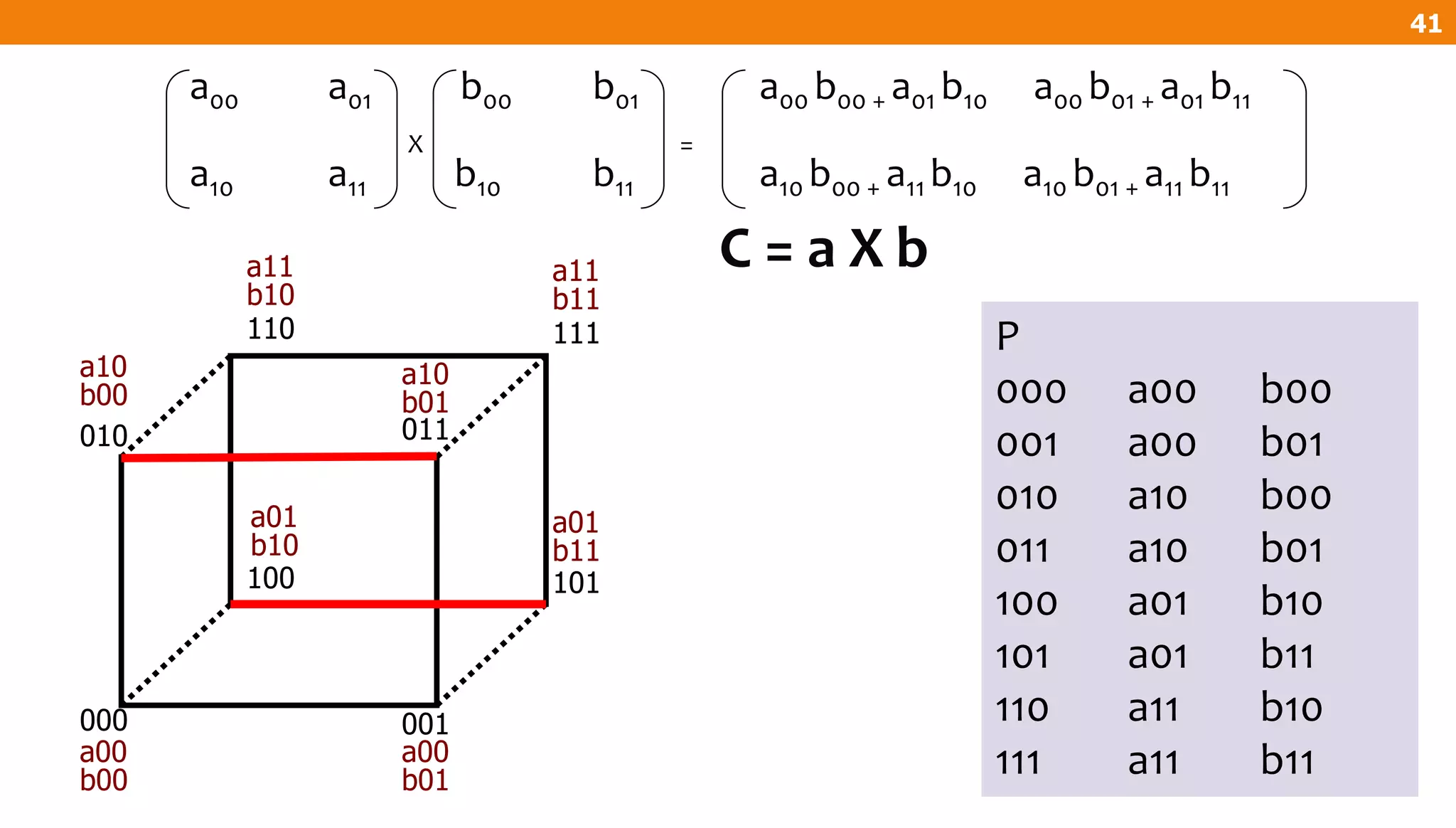
![For all Pm
t = BIT_COMP(m,2)
s = [t]c c = c + s
P
000 a00 b00 a01 b10
001 a00 b01 a01 b11
010 a10 b00 a11 b10
011 a10 b01 a11 b11
100 a01 b10 a00 b00
101 a01 b11 a00 b01
110 a11 b10 a10 b00
111 a11 b11 a10 b01
100 101
110
111
000 001
010 011
a00,b00 a00,b01
a10,b00 a10,b01
a01,b10
a11,b10
a11,b11
a01,b11
Matrix Multiplication on Hypercube
42](https://image.slidesharecdn.com/chapter-7-201007184022/75/Chapter-7-Matrix-Multiplication-42-2048.jpg)