INTRODUCTION TO PARALLEL PROCESSING

By GS kosta
INTRODUCTION TO PARALLEL PROCESSING
Parallel computer structures will be
characterized as pipelined computers,array processors, and multiprocessor systems. Several new computing concepts,including data
flow and VLSI approaches.
1.1 EVOLUTION OF COMPUTER SYSTEMS
physically marked by the rapid changing of building blocks from relays and vacuum tubes (l940-1950s) to discrete diodes and
transistors (1950 1960s), to small- and medium-scale integrated (SSI/MSI) circuits (l960-1970s), and to large- and very-large-scale
integrated (LSI/VLSI) devices (1970s and beyond).Increases in device speed and reliability and reductions in hardware cost and
physical size have greatly enhanced computer performance
1.1.1 Generations of Computer Systems
The first generation (1938-1953)The introduction of the first electronic analog computer in 1938 and the first electronic
digital computer, ENIAC (Electronic Numerical Integrator and Computer), in 1946 marked the beginning of the first
generation of computers. Electromechanical relays were used as switching devices in the 1940s, and vacuumtubes were
used in the 1950s.
The second generation (1952-1963)Transistors were invented in 1948. The first transistorized digital computer, TRAD!C, was
built by Bell Laboratories in 1954.Discrete transistors and diodes were the building blocks: 800 transistors were
used in TRADIC. Printed circuits appeared
The third generation (1962-1975)This generation was marked by the use of small-scale integrated (SSI) and medium-scale
integrated (MSI) circuits as the basic building blocks. Multilayered printed circuits were used.Core memory was
still used in CDC-6600 and other machines but. by 1968, many fast computers, like CDC-7600, began to replace cores with solid-
state memories.
The fourth generation (1972-present) The present generation computers emphasize the use of large-scale integrated (LSI) circuits
for both logic and memory sections. High-density packaging has appeared. High-level languages are being extended to handle both
scalar and vector data. like the extended Fortran in many vector processors,
The future Computers to be used in the 1990s may be the next generation. Very large-scale integrated (VLSI) chips will be used
along with high-density modular design.Multiprocessors like the 16 processors in the S-1 project at Lawrence Livermore National
Laboratory and in the Denelcor's HEP will be required.Cray-2 is expected to have four processors,to be delivered in 1985. More
than 1000mega floating point operations persecond(megaflops) are expected in these future supercomputers.
1.1.2 TrendsTowardsParallel Processing **
According to Sidney Fern Bach:" Today's large computers (mainframes)wouldhere beenconsidered 'supercomputers' 10to 20
years ago.By the same token,today's supercomputers willhe considered'state-of-the-art' standard equipment 10 to 20_yearsFrom
now." from an application point of view. the mainstream usage of computers is experiencing a trend of four ascending
levels of sophistication:
• Data processing
• Information processing • Knowledge processing • Intelligence processing

By GS kosta
We are in an era which is promoting the use ofcomputers not only for conventionaldata-information processing.but also towardthe
building of workable machine knowledge-intelligence systems to advance human civilization. Many computer scientists feel that the
degree of parallelism exploitable at the two highest processing levels should be higher than that at thedata-information processing
levels
From an operating systempoint of view, computer systems have improved chronologically in four phases:
• Batch processing
• Multiprogramming
• Time sharing
• Multiprocessing
In these four operating modes. the degree of parallelism increases sharply from phase to phase.The general trend is to emphasize
parallel processing of information. In what follows. the term information is used with an extended meaning to include
data, information, knowledge, and intelligence. We formally define parallel processing as follows:
Parallel processing is an efficient form of information processing which emphasizes the exploitation of concurrent events in the
computing process.Concurrency implies parallelism, simultaneity, and pipelining. Parallel events may occur in multiple resources
during the same time interval; simultaneous events may occur at the same time instant; and pipelined events may occur in
overlapped time spans.
parallelprocessing can be challenged in four programmatic levels:
• Job or program level
• Task or procedure level
• Interinstruction level
• Intrainstructionlevel The highest job level is often conducted algorithmically. The lowest intrainstruction level is often
implemented directly by hardware means. Hardware roles increase from high to low levels. On the other hand,software
implementations increase from low to high levels. The trade-off between hardware and software approaches to solve a problem is
always a very controversial issue.As hardware cost declines and software cost increases, more and more hardware methods are
replacing the conventionalsoftware approaches.The trend is also supported by the increasing demand for a faster real-time,
resource-sharing, and fault-tolerant computing environment.
parallel processing is concerned,the general architectural trend is being shiftedaway from conventional uniprocessor systems to
multiprocessor systems orto an array of processing elements controlled by one uniprocessor.In all cases,a high degree of pipe
lining is being incorporated into the various systemlevels.
1.2 P ARALLEUSM IN UNIPROCESSOR SYSTEMS
1.2.1 Basic Uniprocessor Architecture
A typical uniprocessor computer consists of three major components: the main memory, the central processing unit
(CPU),and the input-output (l/O) subsystem.

By GS kosta
The architectures of two commercially available uniprocessor computers are given below to show the possible
interconnection of structures among the three subsystems. We will examine majorcomponents in the CPU and in
the 1/0 subsystem.
1.2.2 Parallel Processing Mechanisms
A numberof parallel processingmechanisms havebeendeveloped in uniprocessor computers.We identify them in the following six
categories:
• Multiplicity of functional units
• Parallelism and pipelining within the CPU
• Overlapped CPU and I/0 operations
• Use of a hierarchical memory system
• Balancing of subsystembandwidths
• Multiprogramming and time sharing
Multiplicity of functional units The early computer had only one arithmetic and logic unit in its CPU. Furthermore. the ALU could
only perform one function at a time, a rather slowprocess for executing a long sequence of arithmetic logic instructions.In practice,
many of the functions of the ALU can be distributed to multiple and specialized functional units which can operate in paralle l. The
CDC-6600 (designed in 1964) has I 0 functional units built into its CPU (Figure 1.5). These I 0 units are independent of each other
and may operate simultaneously. A scoreboard is used to keep track of the availability of the functional units and
registers being demanded. With 10 functional units and 24 registers available, the
instructionissue rate canbe significantlyincreased.
Anothergood example of a multifunction uniprocessoris the IBM 360/91 (1968), which has two parallel execution units
Parallelism and pipelining within the CPU Parallel
adders,using such techniques as carry-lookahead and
carry-save, arc now built into almost all ALUs. This is in
contrast to the bit-serial adders used in the first-generation
machines. High-speed multiplier recoding and
convergence division arc techniques for exploring
parallelism and the sharing of hardware resources for the
functions of multiply and divide The use of multiple
functional units is a form of parallelism with the CPU.
Various phases of instruction executions arc now
pipelined, including instruction fetch, decode,operand
fetch, arithmetic logic execution, and store result. To
facilitate overlapped instruction executions through the
pipe, instruction prefetch and data buffering techniques
have been developed.

By GS kosta
Overlapped CPU and 1/0 operations 1/0 operations can be performed simultaneously with the CPU computations by using
separate 1/0 controllers, channels, or I/0 processors.The direct-memory-access (DMA) channel can be used to provide direct
information transfer between the 1/0 devices and the main memory. The DMA is conducted on a cycle-stealingbasis,which is
apparent to the CPU.
Use of hierarchical memory system Usually, the CPU is
about 1000 times faster than memory access.A
hierarchical memory systemcan be used to close up the
speed gap. Computer memory hierarchy is conceptually
illustrated in Figure 1.6.The innermost level is the register
files directly addressable by ALU. Cache memory can be
used to serve as a buffer between the CPU and the main
memory. Block access of the main memory can be
achieved through multi way inter leaving across parallel
memory modules (see Figure 1.4). Virtual memory space
can be established with the use of disks and tape units at
the outerlevels.
Multiprogramming and Time Sharing
Multiprogramming Within the same time interval, there
may be multiple processes active in a computer.
competing for memory. 1/0. and CPG resources.We are
aware of the fact that some computer programs are CPU-
hound (computation intensive),and some are I/O-bound
(input-output intensive)
Time sharing Multiprogramming on a uniprocessoris
centered around the sharing of the CPU by many programs. Sometimes a high-priority program may occupy
the CPU for too long to allow others to share.This problem can be overcome by using a rime-sharingoperating system.
1.3 PARALLEL COMPUTER STRUCTURES
Parallel computers are those systems that emphasize parallel processing.The basic architectural features of parallel computers are
introduced below.' We divide parallel computers into three architectural configurations:
• Pipeline computers
• Array processors
• Multiprocessor systems
A pipeline computer performs overlapped computations to exploit temporal parallelism An array processoruses multiple
synchronized arithmetic logic units to achieve spatial parallelism. A multiprocessor systemachieves asynchronous parallelism
through a setof interactive processors withsharedresources (memories,
database,etc.).
1.4 ARCHITECTURAL CLASSIFICATION SCHEMES
Three computer architectural classification schemes are presented in this section .Flynn'., classification (1966) is based on the
multiplicity of instruction streams and data streams in a computer system. F eng's scheme (1972) is based on serial versus
parallel processing. handler’s classification (1977) is determined by the degree of parallelism and pipelining in various subsystem
levels.
1.4.1 Multiplicity of Instruction-Data Streams
In general, digital computers may be classified into four categories, according to the multiplicity of instruction and data
streams. This scheme for classifying computer organizations was introduced by Michael J. Flynn.
• Computer organizations are characterized by the
multiplicity of the hardware provided to service
the instruction and data streams. Listed below
are Flynn's four machine organizations:
• Single instruction stream-single data stream
(SISD)
• Single instruction stream-multiple data
stream (SIMD)
• Multiple instruction stream-single data
stream (MISD)
• Multiple instruction stream-multiple data
stream (MI MD)

By GS kosta
SISD computer organization This organization, shown in figure 1.16a, represents most serial computers available today.
Instructions are executed sequentially but may be overlapped in their execution stages (pipelining). Most SISD uniprocessor
systems are pipelined. An SISD computer may have more than one functional unit in it. All the functional units are under the
supervision of one control unit.
SIMD computer organization This class corresponds to array processors.Introduced in Section 1.3.2. As illustrated in Figure
1.16b, there are multiple processing elements supervised by the same control unit. All PEs receive the same instruction broad cast
from the control unit but operate on different data sets from distinct data streams. The shared memory subsystemmay contain
multiple modules.
MISD computer organization This organization is conceptually illustrated in Figure l.l6c. There are n processorunits, each
receiving distinct instructions operating over the same data stream and its derivatives. The results (output)of one processorbec ome
the input (operands) of the next processorin the micropipe. This structure has received much less attention and has been cha llenged
as impractical by some computer architects.No real embodiment of this class exists.
MIMD computer organization Most multiprocessor systems and multiple computer systems can be classified in this category
(Figure 1.16d). An intrinsic MIMDcomputer implies
interactions among then processors because all memory
streams are derived from the same data space shared by
all processors.If the n data streams were derived from
disjointed subspaces ofthe shared memories, then we
would have the so-called multiple SISD (MSISD)
operation, which is nothing but a set of n
independent SISD uniprocessorsystems.
1.4.2 Serial Versus Parallel Processing
Tse-yun Feng has suggested the use ofthe degree of
parallelism to
classify various
computer
architectures.
There are four types of processing methods that can be seen from this diagram:
• Word-serial and bit-serial (WSBS)
• Word-parallel and bit-serial (WPBS)
• Word-serial and bit-parallel (WSBP)

By GS kosta
• Word-parallel and bit-parallel (WPBP)
WSBS has been called bit-serial processing because one bit (n = m = 1) is processed at a time. a rather slow process.This was
done only in the first~generationcomputers.WPBS (n = 1, m > 1) has been called bis (bit-slice) processin9 because an m-bit slice is
processed at a time. WSBP (n > 1, m = l ), as found in most existing computers, has been called word-slice processi11g because one
word of 11 bits is processed at a time. Finally, WPBP (n > I, m > l) is known as fully parallel processing(orsimply parallel
processing,if no confusion exists), in which an array of n · m bits is processed at one time, the fastest processing mode of the four.
In Table 1.4, we have listed a number of computer systems undereach processing mode. The sys temparameters n, m are also shown
for each system.The bit-slice processors,like STARAN. ~PP, and DAP. all have long bit slices. llliac-IV and PEPE are two word-
slice array processors.
1.4.3 Parallelism Versus Pipelining
Wolfgang Handler has proposed a classification scheme for identifying the parallelism degree and pipe lining degree built into the
hardware structures of a computer system.He considers parallel-pipeline processing at three subsystemlevels:
• Processorcontrol unit (PCU)
• Arithmetic logic unit (ALU)
• Bit-level circuit (BLC)
The functions of PCU and ALU should be clear to us.Each PCU corresponds to one processoror one CPU. The ALU is equivalent
to the processing element (PE)we specified for SIMD array processors.The BLC corresponds to the combinational logic circuitry
needed to perform !-bit operations in the ALU. A computer systemC can be characterized by a triple containing six independent
entities. as defined below:
T(C) = < K x K', D x D', W x W'> (1.13)
where K = the number of processors (PCUs) within the computer
D = the number of ALUs (or PEs) under the control of one PCU
W = the word length of an ALU or of a PE
W' =the number of pipeline stages in all ALUs or in a PE
D' = the number of ALUs that can be pipelined (pipeline chaining to be
described in Chapter 4)
K' = the number of PCUs that can be pipelined
Several real computer examples are used to clarify the above parametric descriptions.The Texas Instrument's Advanced Scientific
Computer (Tl-ASC)has one controller controlling four arithmetic pipelines, each has 64-bit word lengths and eight stages.Thus,we
have
T(ASC) = <1 x 1, 4 X 1, 64 x 8> = < 1, 4, 64 x 8>

By GS kosta
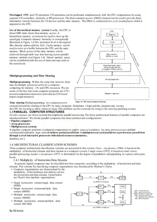
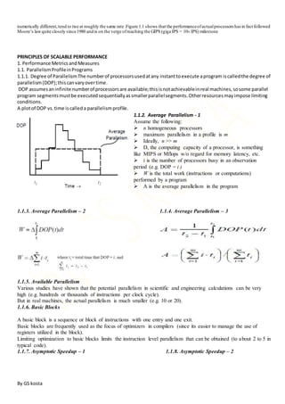
Amdahl's law
In computer architecture, Amdahl's law (or Amdahl's
argument[1]
) is a formula which gives the
theoretical speedup in latency of the execution of a
task at fixed workload that can be expected of a
system whose resources are improved. It is named
after computer scientist Gene Amdahl, and was
presented at the AFIPS Spring Joint Computer
Conference in 1967
Amdahl's law is often used in parallel computing to
predict the theoretical speedup when using multiple
processors.
Amdahl's law applies only to the cases where the
problem size is fixed.

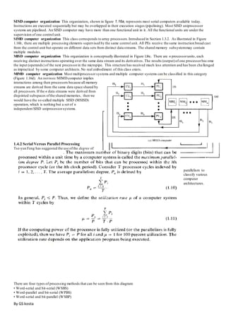
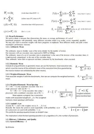
By GS kosta
Moore’s Law
The quest for higher-performance digital computers seems unending. In
the past two decades,the performance ofmicroprocessors has enjoyed an
exponentialgrowth.The growth ofmicroprocessorspeed/performanceby
a factor of 2 every 18 months (or about 60% per
year)is known as Moore’slaw.This growth is the result ofa combination
of two factors:
1. Increase in complexity (related both to higher device density and to
larger size) ofVLSI chips,projectedto rise to around 10M transistors per
chip for microprocessors, and 1B for dynamic random-access memories
(DRAMs), by the year 2000 [SIA94]
2. Introductionof,andimprovementsin,architectural features suchas on-
chip cache memories, large instruction buffers, multiple instruction issue
per cycle, multithreading, deep pipelines, out-of-order instruction
execution, and branch prediction
Moore’s lawwas originally formulated in 1965 in terms ofthe doubling
of chip complexity every year(laterrevised to every 18months)based
only on a small numberof data points[Scha97].Moore’srevised
prediction matchesalmost perfectly the actualincreasesin the
number of transistors in DRAM and microprocessor chips.
Moore’s lawseems to hold regardlessofhowone measures
processorperformance:counting the numberofexecuted
instructionspersecond(IPS),counting the numberoffloating-point
operationspersecond (FLOPS),or using sophisticatedbenchmark
suites thatattempt to measure theprocessor'sperformance onreal
applications.This is because allof these measures,though
Figure 1.1. The exponential grow th of microprocessor performance,
know n as Moore’s law , show n overthe past two decades.

By GS kosta
numerically different,tend to rise at roughly the same rate .Figure 1.1 shows that the performanceofactualprocessors has in fact followed
Moore’s lawquite closely since1980 and is on the verge ofreaching the GIPS (giga IPS = 109 IPS) milestone
PRINCIPLES OF SCALABLE PERFORMANCE
1. Performance MetricsandMeasures
1.1. ParallelismProfileinPrograms
1.1.1. Degree of ParallelismThe numberof processorsusedatany instanttoexecute aprogram iscalledthe degree of
parallelism(DOP);thiscanvaryovertime.
DOP assumesaninfinite numberof processorsare available;thisisnotachievableinreal machines,sosome parallel
program segmentsmustbe executedsequentiallyassmallerparallelsegments.Otherresourcesmayimpose limiting
conditions.
A plotof DOP vs.time iscalleda parallelismprofile.
1.1.2. Average Parallelism - 1
Assume the following:
n homogeneous processors
maximum parallelism in a profile is m
Ideally, n >> m
D, the computing capacity of a processor, is something
like MIPS or Mflops w/o regard for memory latency, etc.
i is the number of processors busy in an observation
period (e.g. DOP = i )
W is the total work (instructions or computations)
performed by a program
A is the average parallelism in the program
1.1.3. Average Parallelism – 2 1.1.4. Average Parallelism – 3
1.1.5. Available Parallelism
Various studies have shown that the potential parallelism in scientific and engineering calculations can be very
high (e.g. hundreds or thousands of instructions per clock cycle).
But in real machines, the actual parallelism is much smaller (e.g. 10 or 20).
1.1.6. Basic Blocks
A basic block is a sequence or block of instructions with one entry and one exit.
Basic blocks are frequently used as the focus of optimizers in compilers (since its easier to manage the use of
registers utilized in the block).
Limiting optimization to basic blocks limits the instruction level parallelism that can be obtained (to about 2 to 5 in
typical code).
1.1.7. Asymptotic Speedup – 1 1.1.8. Asymptotic Speedup – 2

By GS kosta
1.2. Mean Performance
We seek to obtain a measure that characterizes the mean, or average, performance of a set of
benchmark programs with potentially many different execution modes (e.g. scalar, vector, sequential, parallel).
We may also wish to associate weights with these programs to emphasize these different modes and yield a more
meaningful performance measure.
1.2.1. Arithmetic Mean
The arithmetic mean is familiar (sum of the terms divided by the number of terms).
Our measures will use execution rates expressed in MIPS or Mflops.
The arithmetic mean of a set of execution rates is proportional to the sum of the inverses of the execution times; it
is not inversely proportional to the sum of the execution times.
Thus arithmetic mean fails to represent real times consumed by the benchmarks when executed.
1.2.2. Harmonic Mean
Instead of using arithmetic or geometric mean, we use the harmonic mean execution rate,
which is just the inverse of the arithmetic mean of the executiontime (thus guaranteeing
the inverse relation not exhibitedby the other means).
1.2.3. Weighted Harmonic Mean
If we associate weights fi with the benchmarks, then we can compute the weighted harmonic
mean:
1.2.4. Weighted Harmonic Mean Speedup
T1 = 1/R1 = 1 is the sequential execution time on a
single processor with rate R1 = 1.
Ti = 1/Ri = 1/i = is the execution time using i
processors with a combined execution rate of Ri = i.
Now suppose a program has n execution
modes with associated weights f1 … f n. The w eighted
harmonic mean speedup is definedas:
1.2.5. Amdahl’s Law
Assume Ri = i, and w (the weights) are (a, 0, …, 0, 1-a).
Basically this means the system is used sequentially (with probability a) or
all n processors are used (with probability 1- a).
This yieldsthe speedup equation known as Amdahl’s law:
The implication is that the best speedup possible is 1/ a, regardless of n, the number of processors.
1.3. Efficiency, Utilizations, and Quality
1.3.1. System Efficiency – 1

By GS kosta
Assume the following definitions:
O (n) = total number of “unit operations” performed by an n processor system in completing a program P.
T (n) = execution time required to execute the program P on an n processor system.
O (n) can be considered similar to the total number of instructions executed by the n processors, perhaps scaled by
a constant factor.
If we define O (1) = T (1), then it is logical to expect that T (n) < O (n) when n > 1 if the program P is able to make
any use at all of the extra processor(s).
1.3.2. System Efficiency – 2
Clearly, the speedup factor (how much faster the program runs with n processors) can now be expressed as
S (n) = T (1) / T (n)
Recall that we expect T (n) < T (1), so S (n) ³ 1.
System efficiency is defined as
E (n) = S (n) / n = T (1) / ( n ´ T (n) )
It indicates the actual degree of speedup achieved in a system as compared with the maximum possible speedup.
Thus 1 / n £ E (n) £ 1. The value is 1/n when only one
processor is used (regardless of n), and the value is 1 when all processors are fully utilized.
1.3.3. Redundancy
The redundancy in a parallel computation is defined as
R (n) = O (n) / O (1)
What values can R (n) obtain?
R (n) = 1 when O (n) = O (1), or when the number of operations performed is independent of the number of
processors, n. This is the ideal case.
R (n) = n when all processors performs the same number of operations as when only a single processor is used; this
implies that n completely redundant computations are performed!
The R (n) figure indicates to what extent the software parallelismis carried over to the hardware implementation
without having extra operations performed.
1.3.4. System Utilization
System utilization is defined as
U (n) = R (n) xE (n) = O (n) / ( nxT (n) )
It indicates the degree to which the system resources were kept busy during execution of the
program. Since 1 £ R (n) £ n, and 1 / n £ E (n) £
1, the best possible value for U (n) is 1, and the
worst is 1 / n.
SPEEDUP PERFORMANCE LAWS
The main objective is to produce the results as early as possible. In other words minimal turnaround time is the
primary goal.
Three performance laws defined below:
1. Amdahl’s Law(1967) is based on fixed workload or fixed problem size
2. Gustafson’s Law(1987) is applied to scalable problems, where the problem size increases with the increase in
machine size.
3. The speed up model by Sun and Ni(1993) is for scaled problems bounded by memory capacity.
Amdahl’s Law for fixed workload
In many practical applications the computational workload is often fixed with a fixed problem size. As the number
of processors increases, the fixed workload is distributed.
Speedup obtained for time-critical applications is called fixed-load speedup.
Fixed-Load Speedup

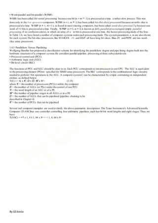
By GS kosta
The ideal speed up formula given below:
is based on a fixed workload, regardless of machine size.
We consider below two cases of DOP< n and of DOP ≥ n.
Parallel algorithm
In computer science, a parallel algorithm, as opposed to a traditional serial algorithm, is an algorithm which can
be executed a piece at a time on many different processing devices, and then combined together again at the end
to get the correct result.[1]
Many parallel algorithms are executed concurrently – though in general concurrent algorithms are a distinct
concept – and thus these concepts are often conflated, with which aspect of an algorithm is parallel and which is
concurrent not being clearly distinguished. Further, non-parallel, non-concurrent algorithms are often referred to
as "sequential algorithms", by contrast with concurrent algorithms.
Examples of Parallel Algorithms
This section describes and analyzes several parallel algorithms. These algorithms provide examples of how to analyze algorithms in terms of work
and depth and of how to use nested data-parallel constructs. They also introduce some important ideas concerning parallel algorithms. We mention
again that the main goals are to have thecode closely match the high-level intuition of the algorithm, and to make it easy to analyzethe asymptotic
performance from the code.
Parallel Algorithm Complexity
Analysis of an algorithm helps us determine whether the algorithm is useful or not. Generally, an algorithm is analyzed based on its
execution time (Time Complexity) and the amount of space (Space Complexity) it requires.
Since we have sophisticated memory devices available at reasonable cost, storage space is no longer an issue. Hence, spa ce
complexity is not given so much of importance.
Parallel algorithms are designed to improve the computation speed of a computer. For analyzing a Parallel Algorithm, we norma lly
consider the following parameters −
 Time complexity (Execution Time),

By GS kosta
 Totalnumber of processors used, and
 Totalcost.
Time Complexity
The main reason behind developing parallel algorithms was to reduce the computation time of an algorithm. Thus, evaluating th e
execution time of an algorithm is extremely important in analyzing its efficiency.
Execution time is measured on the basis of the time taken by the algorithm to solve a problem. The total execution time is calculated
from the moment when the algorithm starts executing to the moment it stops.If all the processors do not start or end execution at the
same time, then the total execution time of the algorithm is the moment when the first processorstarted its execution to the moment
when the last processor stops its execution.
Time complexity of an algorithm can be classified into three categories−
 Worst-case complexity − When the amount of time required by an algorithm for a given input is maximum.
 Average-case complexity − When the amount of time required by an algorithm for a given input is average.
 Best-case complexity − When the amount of time required by an algorithm for a given input is minimum.
Asymptotic Analysis
The complexity or efficiency of an algorithm is the number of steps executed by the algorithm to get the desired output.Asymptotic
analysis is done to calculate the complexity of an algorithm in its theoretical analysis. In asymptotic analysis,a large length of input
is used to calculate the complexity function of the algorithm.
Note − Asymptotic is a condition where a line tends to meet a curve, but they do not intersect. Here the line and the curve is
asymptotic to each other.
Asymptotic notation is the easiest way to describe the fastest and slowest possible execution time for an algorithm using hig h bounds
and low bounds on speed. For this, we use the following notations −
 Big O notation
 Omega notation
 Thetanotation
Big O notation
In mathematics, Big O notation is used to represent the asymptotic characteristics offunctions.It represents the behavioro fa function
for large inputs in a simple and accurate method. It is a method of representing the upper bound of an algorithm’s execution time. It
represents the longest amount of time that the algorithm could take to complete its execution. The function −
f(n) = O(g(n))
iff there exists positive constants c and n0 such that f(n) ≤ c * g(n) for all nwhere n ≥ n0.
Omega notation
Omega notation is a method of representing the lower bound of an algorithm’s execution time. The function −
f(n) = Ω (g(n))
iff there exists positive constants c and n0 such that f(n) ≥ c * g(n) for all nwhere n ≥ n0.
Theta Notation
Theta notation is a method of representing both the lower bound and the upper bound of an algorithm’s execution time. The function
−
f(n) = θ(g(n))
iff there exists positive constants c1, c2, and n0 such that c1 * g(n) ≤ f(n) ≤ c2 * g(n) for all n where n ≥ n0.
Speedup of anAlgorithm
The performance of a parallel algorithm is determined by calculating its speedup. Speedup is defined as the ratio of the worst-case
execution time of the fastest known sequential algorithm for a particular problem to the worst-case execution time of the parallel
algorithm.
speedup = Worst case execution time of the fastest known sequential for a particular problem / Worst case execution time of theparallel
algorithm

By GS kosta
Number of ProcessorsUsed
The number of processors used is an important factor in analyzing the efficiency of a parallel algorithm. The cost to buy, ma intain,
and run the computers are calculated. Larger the number of processors used by an algorithmto solve a problem, more costly becomes
the obtained result.
Total Cost
Total cost of a parallel algorithm is the product of time complexity and the number of processors used in that particular alg orithm.
Total Cost = Time complexity × Number of processors used
Therefore, the efficiency of a parallel algorithm is –
Efficiency = Worst case execution time of sequential algorithm / Worst case execution time of the parallel algorithm
Models of Parallel Processing
Parallel processors come in manydifferentvarieties.
1. SIMD VERSUS MIMD ARCHITECTURES
Within the SIMD category, two fundamental design choices exist:
1. Synchronous versus asynchronous SIMD. In a SIMD machine, each processor can execute or ignore the instruction being broadcast
based on its local stateor data-dependent conditions. However, this leads to some inefficiency in executing conditional computations.
For example, an “if-then-else” statement is executed by first enabling the processors for which the condition is satisfied and then flipping
the “enable” bit before getting into the “else” part. On the average, half of the processors will be idle for each branch. The situation is
even worsefor “case” statements involving multiway branches. A possiblecure is to use the asynchronous version of SIMD, known as
SPMD (spim-dee or single-program, multiple data), where each processor runs its own copy of the common program. Theadvantage of
SPMD is that in an “if-then-else” computation, each processor will only spend time on the relevant branch. The disadvantages include
the need for occasional synchronization and the higher complexity of each processor, which must now have a program memory and
instruction fetch/decode logic.
2. Custom- versus commodity-chip SIMD. A SIMD machine can be designed based on commodity (off-the-shelf) components or with
custom chips. In the first approach, components tend to be inexpensive because of mass production. However, such general-purpose
components will likely contain elements that may not be needed for a particular design. These extra components may complicate the
design, manufacture, and testing of theSIMD machine and may introduce speed penalties as well. Customcomponents (including ASICs
= application-specificICs, multichip modules, or WSI = wafer-scale integrated circuits) generally offer better performance but lead to
much higher cost in view of their development costs being borne by a relatively small number of parallel machine users (as op posed to
commodity microprocessors that are produced in millions). As integrating multiple processors along with ample memory on a single
VLSI chip becomes feasible, a typeof convergence between the two approaches appears imminent.
Within the MIMD class, three fundamental issuesor design choices are subjects of ongoing debates in the research community:
1. MPP—massively ormoderatelyparallel processor. Is it more cost-effective to build a parallelprocessorout ofa relatively small
numberof powerfulprocessorsora massive numberofvery simple processors (the“herd ofelephants” orthe “army ofants”
approach)? Referring to Amdahl’s law,the first choice does betteron the inherently sequentialpart ofa computation while the
secondapproach might allowa higherspeed-upforthe parallelizable part.A generalanswercannot be given to this question,as
the best choiceis both application-and technology-dependent.
2. Tightly versusloosely coupled MIMD. Which is a betterapproach to high-performance computing,thatofusing specially
designedmultiprocessors/multicomputerora collection ofordinary workstations thatare interconnected by commoditynetworks
(such as EthernetorATM)and whose interactions are coordinated byspecialsystemsoftware anddistributed file systems? The
latterchoice,sometimes referred to as network ofworkstations (NOW)orclustercomputing,has beengainingpopularity in
recent years.However,many open problems exist fortaking full advantage ofsuch network-based loosely coupled architectures.
The hardware,systemsoftware,and applications aspects ofNOWs are being investigated by numerous researchgroups.
3. .Explicit message passing versusvirtualshared memory. Which scheme is better,that offorcing the users to explicitly specify all
messagesthatmust be sent betweenprocessors orto allowthemto programin an abstracthigher-levelmodel,with the required
messagesautomatically generated bythe systemsoftware? This question is essentially very similar to the one asked in the early
days ofhigh-levellanguages and virtualmemory.At some point in the past,programming in as sembly languages anddoing
explicit transfers betweensecondary andprimary memories could lead to higherefficiency.However,nowadays,software is so
complex and compilers and operating systems so advanced (notto mention processingpowerso cheap)that it no longermakes
sense to hand-optimize the programs,except in limited time-critical instances.However,we are not yet at that point in parallel
processing,and hiding the explicit communication structure ofa parallel machine fromthe programmer has nontrivial
consequencesforperformance

By GS kosta
THE PRAM SHARED-MEMORY MODEL
The theoretical model used for conventional or sequential computers (SISD class) is
known as therandom-access machine (RAM) (not to be confused with random-access
memory, which has the same acronym). Theparallel version of RAM [PRAM (pea-ram)],
constitutes an abstract model of the class of global-memory parallel processors. The
abstraction consists of ignoring the details of the processor-to-memory interconnection
network and taking theview that each processor can access any memory location in each
machine cycle, independent of what other processors are doing
DISTRIBUTED-MEMORY OR GRAPH MODELS
This network is usually represented as a graph, with vertices corresponding to processor–memory nodes and edges corresponding to
communication links. If communication links are unidirectional, then directed edges are used. Undirected edges imply bidirectional
communication, although not necessarily in both directions at once. Important parameters of an interconnection network include
1. Network diameter: thelongest of the shortest paths
between various pairs of nodes, which should be
relatively small if network latency is to be minimized.
The network diameter is more important with store-and-
forward routing (when a message is stored in its entirety
and retransmitted by intermediate nodes) than with
wormhole routing (when a message is quickly relayed
through a node in small pieces).
2. Bisection (band)width: thesmallest number (total
capacity) of links that need to be cut in order to divide
the network into two subnetworks of half the size. This
is important when nodes communicate with each other
in a random fashion. A small bisection (band)width
limits the rate of data transfer between thetwo halves of
the network, thus affecting theperformance of
communication-intensive algorithms.
3. Vertex or node degree: the number of communication
ports required of each node, which should be a constant
independent of network size if the architecture is to be
readily scalable to larger sizes. Thenode degree has a
direct effect on thecost of each node, with the effect
being more significant for parallel ports containing
several wires or when the node is required to
communicate over all of its ports at once.
CIRCUIT MODEL AND PHYSICAL REALIZATIONS
In a sense, the only sure way to predict the performance of a parallel architecture on a
given set of problems is to actually build themachine and run the programs on it. Because
this is often impossible or very costly, the next best thing is to model themachine at the
circuit level, so that all computationaland signal propagation delays can be taken into
account. Unfortunately, this is also impossible for a complex supercomputer, both because
generating and debugging detailed circuit specifications are not much easier than a
fullblown
implementation and because a circuit simulator would take eons to run the simulation.
Despitetheabove observations, we can produce and evaluate circuit-level designs for
specific applications.
GLOBAL VERSUS DISTRIBUTED MEMORY
Within the MIMDclass ofparallelprocessors,memory can be globalordistributed.
Global memory may be visualized as being in a central location where all processors can
access it with equal ease (or with equal difficulty, if you are a half-empty-glass typeof
person). Figure 4.3 shows a possiblehardware organization for a global-memory parallel
processor. Processors can access memory through a special processor-to-memory network.
A global-memory multiprocessor is characterized by the typeand number p of processors,
the capacity and number m of memory modules, and the network architecture. Even though
p and m are independent parameters, achieving high performance typically requires that they
be comparable in magnitude (e.g., too few memory modules will cause contention among
the processors and too many would complicate the network design).

By GS kosta
Distributed-memory architectures can be conceptually viewed as in Fig. 4.5. A collection of p processors, each with its own privatememory,
communicates through an interconnection network. Here, the latency of the
interconnection network may be less critical, as each processor is likely to
access its own local memory most of the time. However, the communication
bandwidth of thenetwork may or may not be critical, depending on the typeof
parallel applications and the extent of task interdependencies. Note that each
processor is usually connected to thenetwork through multiple links or channels
(this is the norm here ,although it can also be the case for shared-memory
parallel processors).
Cache coherence
In computer architecture, cache coherence is the uniformity
of shared resource data that ends up stored in multiple local
caches. When clients in a system maintain caches of a
common memory resource, problems may arise with
incoherent data, which is particularly the case with CPUs in
a multiprocessingsystem.
In the illustration on the right, consider both the clients have
a cached copy of a particular memory block from a previous
read. Suppose the client on the bottom updates/changes
that memory block, the client on the top could be left with an
invalid cache of memory without any notification of the
change. Cache coherence is intended to manage such
conflicts by maintaining a coherent view of the data values in
multiple caches.
The following are the requirements for cache coherence:[2]
Write Propagation
Changes to the data in any cache must be propagated to other copies(of that cache line) in the peer
caches.
Transaction Serialization
Reads/Writes to a single memory location must be seen by all processors in the same order.
Coherence protocols
Coherence Protocols apply cache coherence in multiprocessor systems. The intention is that two clients must
never see different values of the same shared data.
The protocol must implement the basic requirements for coherence. It can be tailor made for the target
system/application.
Protocols can also be classified as Snooping(Snoopy/Broadcast) or Directory based. Typically, early systems
used directory based protocols where a directory would keep a track of the data being shared and the sharers. In
Snoopy protocols , the transaction request. (read/write/upgrade) are sent out to all processors. All processors
snoop the request and respond appropriately.
Write Propagation in Snoopy protocols can be implemented by either of the following:
Write Invalidate
When a write operation is observed to a location that a cache has a copy of, the cache controller
invalidates its own copy of the snooped memory location, and thus forcing reads from main memory of the
new value on their next access.[4]
Write Update
When a write operation is observed to a location that a cache has a copy of, the cache controller updates
its own copy of the snooped memory location with the new data.

By GS kosta
If the protocol design states that whenever any copy of the shared data is changed, all the other copies
must be "updated" to reflect the change, then it is a write update protocol. If the design states that on a
write to a cached copy by any processor requires other processors to discard/invalidate their cached
copies, then it is a write invalidate protocol.
However, scalability is one shortcoming of broadcast protocols.
Various models and protocols have been devised for maintaining coherence.
Parallel Algorithm - Models
The model of a parallel algorithm is developed by considering a strategy for dividing the
data and processing method and applying a suitable strategy to reduce interactions. In
this chapter, we will discuss the following Parallel Algorithm Models −
 Data parallel model
 Task graph model
 Work pool model
 Master slave model
 Producer consumer or pipeline model
 Hybrid model
Data Parallel
In data parallel model, tasks are assigned to processes and each task performs similar
types of operations on different data. Data parallelism is a consequence of single
operations that is being applied on multiple data items.
Data-parallel model can be applied on shared-address spaces and message-passing
paradigms. In data-parallel model, interaction overheads can be reduced by selecting a
locality preserving decomposition, by using optimized collective interaction routines, or
by overlapping computation and interaction.
The primary characteristic of data-parallel model problems is that the intensity of data
parallelism increases with the size of the problem, which in turn makes it possible to
use more processes to solve larger problems.
Example − Dense matrix multiplication.

By GS kosta
Task Graph Model
In the task graph model, parallelism is expressed by a task graph. A task graph can
be either trivial or nontrivial. In this model, the correlation among the tasks are utilized
to promote locality or to minimize interaction costs. This model is enforced to solve
problems in which the quantity of data associated with the tasks is huge compared to
the number of computation associated with them. The tasks are assigned to help
improve the cost of data movement among the tasks.
Examples − Parallel quick sort, sparse matrix factorization, and parallel algorithms
derived via divide-and-conquer approach.
Here, problems are divided into atomic tasks and implemented as a graph. Each task is
an independent unit of job that has dependencies on one or more antecedent task. After

By GS kosta
the completion of a task, the output of an antecedent task is passed to the dependent
task. A task with antecedent task starts execution only when its entire antecedent task
is completed. The final output of the graph is received when the last dependent task is
completed (Task 6 in the above figure).
Work Pool Model
In work pool model, tasks are dynamically assigned to the processes for balancing the
load. Therefore, any process may potentially execute any task. This model is used when
the quantity of data associated with tasks is comparatively smallerthan the computation
associated with the tasks.
There is no desired pre-assigning of tasks onto the processes. Assigning of tasks is
centralized or decentralized. Pointers to the tasks are saved in a physically shared list,
in a priority queue, or in a hash table or tree, or they could be saved in a physically
distributed data structure.
The task may be available in the beginning, or may be generated dynamically. If the
task is generated dynamically and a decentralized assigning of task is done, then a
termination detection algorithm is required so that all the processes can actually detect
the completion of the entire program and stop looking for more tasks.
Example − Parallel tree search
Master-Slave Model
In the master-slave model, one or more master processes generate task and allocate it
to slave processes. The tasks may be allocated beforehand if −

By GS kosta
 the master can estimate the volume of the tasks, or
 a random assigning can do a satisfactory job of balancing load, or
 slaves are assigned smaller pieces of task at different times.
This model is generally equally suitable to shared-address-space or message-
passing paradigms, since the interaction is naturally two ways.
In some cases, a task may need to be completed in phases, and the task in each phase
must be completed before the task in the next phases can be generated. The master-
slave model can be generalized to hierarchical or multi-level master-slave
model in which the top level master feeds the large portion of tasks to the second-level
master, who further subdivides the tasks among its own slaves and may perform a part
of the task itself.
Precautions in using the master-slave model
Care should be taken to assure that the master does not become a congestion point. It
may happen if the tasks are too small or the workers are comparatively fast.
The tasks should be selected in a way that the cost of performing a task dominates the
cost of communication and the cost of synchronization.
Asynchronous interaction may help overlap interaction and the computation associated
with work generation by the master.
Pipeline Model
It is also known as the producer-consumer model. Here a set of data is passed on
through a series of processes, each of which performs some task on it. Here, the arrival
of new data generates the execution of a new task by a process in the queue. The
processes could form a queue in the shape of linear or multidimensional arrays, trees,
or general graphs with or without cycles.
This model is a chain of producers and consumers. Each process in the queue can be
considered as a consumer of a sequence of data items for the process preceding it in
the queue and as a producer of data for the process following it in the queue. The queue
does not need to be a linear chain; it can be a directed graph. The most common

By GS kosta
interaction minimization technique applicable to this model is overlapping interaction
with computation.
Example − Parallel LU factorization algorithm.
Hybrid Models
A hybrid algorithm model is required when more than one model may be needed to
solve a problem.
A hybrid model may be composed of either multiple models applied hierarchically or
multiple models applied sequentially to different phases of a parallel algorithm.
Example − Parallel quick sort
Shared memory/Parallel Processing in Memory
In computer science, shared memory is memory that may be
simultaneously accessed by multiple programs with an intent
to provide communication among them or avoid redundant
copies. Shared memory is an efficient means of passing data
between programs. Depending on context, programs may
run on a single processor or on multiple separate
processors.
Using memory for communication inside a single
program, e.g. among its multiple threads, is also referred
to as shared memory.
In hardware[edit]
In computer hardware, shared memory refers to a (typically large) block of random access memory (RAM) that
can be accessed by several different central processing units (CPUs) in a multiprocessor computer system.
Shared memory systems may use:[1]
 uniform memory access (UMA): all the processors share the physical memory uniformly;
 non-uniform memory access (NUMA): memory access time depends on the memory location relative to a
processor;
 cache-only memory architecture (COMA): the local memories for the processors at each node is used as
cache instead of as actual main memory.
In software[edit]
In computer software, shared memory is either

By GS kosta
 a method of inter-process communication (IPC), i.e. a way of exchanging data between programs running at
the same time. One process will create an area in RAMwhich other processes can access;
 a method of conserving memory space by directing accesses to what would ordinarily be copies of a piece of
data to a single instance instead, by using virtual memorymappings or with explicit support of the program in
question. This is most often used for shared libraries and for XIP.

INTRODUCTION TO PARALLEL PROCESSING

Recommended

Recommended

More Related Content

What's hot

What's hot (20)

Similar to INTRODUCTION TO PARALLEL PROCESSING

Similar to INTRODUCTION TO PARALLEL PROCESSING (20)

Recently uploaded

Recently uploaded (20)

INTRODUCTION TO PARALLEL PROCESSING