Elementary Parallel Algorithms

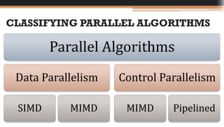
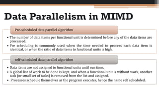
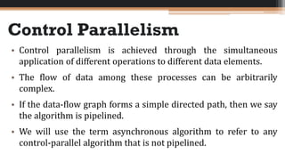
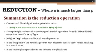
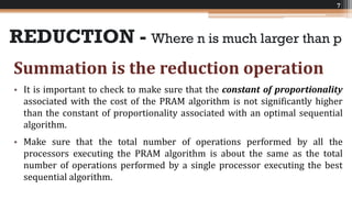
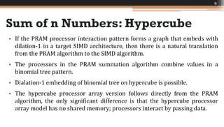
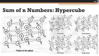
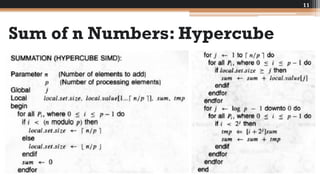
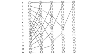
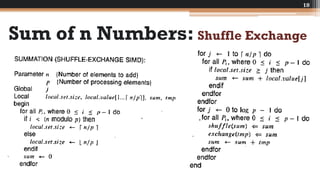
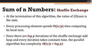
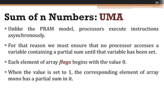
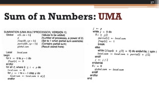
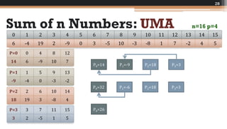
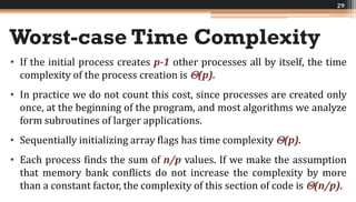
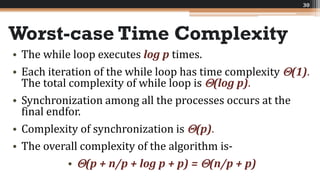
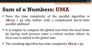
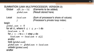
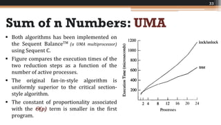
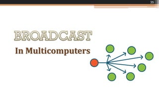
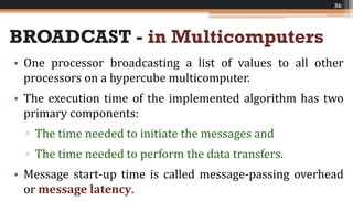
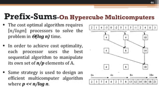
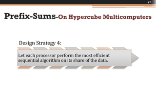
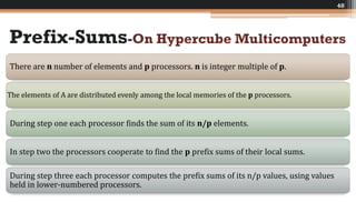
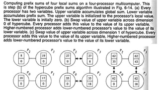
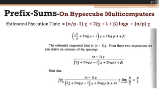
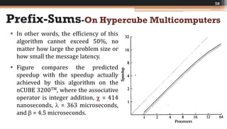
By
Dr. Heman Pathak
Associate Professor
KGC - Dehradun
CHAPTER-6
Parallel Computing
Theory and Practice
By Michel J. Quinn

CLASSIFYING PARALLEL ALGORITHMS
Parallel Algorithms
Data Parallelism
SIMD MIMD
Control Parallelism
MIMD Pipelined

Data Parallelism in MIMD
• The number of data items per functional unit is determined before any of the data items are
processed.
• Pre scheduling is commonly used when the time needed to process each data item is
identical, or when the ratio of data items to functional units is high.
Pre-scheduled data parallel algorithm
• Data items are not assigned to functional units until run time.
• A global list of work to be done is kept, and when a functional unit is without work, another
task (or small set of tasks) is removed from the list and assigned.
• Processes schedule themselves as the program executes, hence the name self scheduled.
self-scheduled data parallel algorithm

Control Parallelism
• Control parallelism is achieved through the simultaneous
application of different operations to different data elements.
• The flow of data among these processes can be arbitrarily
complex.
• If the data-flow graph forms a simple directed path, then we say
the algorithm is pipelined.
• We will use the term asynchronous algorithm to refer to any
control-parallel algorithm that is not pipelined.

REDUCTION
5
• lf a cost optimal CREW PRAM algorithm exists and the way the PRAM processors
interact through shared variables maps onto the target architecture, a PRAM
algorithm is a reasonable staring point.
Design Strategy 1
 Consider the problem of performing a reduction operation on a set of n
values, where n is much larger than p, the number of available
processors.
 Objective is to develop a parallel algorithm that introduces the
minimum amount of extra operations compared to the best sequential
algorithm.

REDUCTION - Where n is much larger than p
6
Summation is the reduction operation
• Cost-optimal PRAM algorithm for global sum exists:
▫ n/ log n processors can add n numbers in (log n) time.
• Same principle can be used to develop good parallel algorithms for real SIMD and MIMD
computers, even if p << n/ log n.
• 𝒏/𝒑 𝒐𝒓 𝒏/𝒑 values are allocated to each processor.
• In the first phase of the parallel algorithm each processor adds its set of values, resulting
in p partial sums.
• In the second phase partial sums are combine into global sum.

REDUCTION - Where n is much larger than p
7
Summation is the reduction operation
• It is important to check to make sure that the constant of proportionality
associated with the cost of the PRAM algorithm is not significantly higher
than the constant of proportionality associated with an optimal sequential
algorithm.
• Make sure that the total number of operations performed by all the
processors executing the PRAM algorithm is about the same as the total
number of operations performed by a single processor executing the best
sequential algorithm.

Hypercube SIMD Model
8
6 7
54
2 3
10

Sum of n Numbers: Hypercube
• If the PRAM processor interaction pattern forms a graph that embeds with
dilation-1 in a target SIMD architecture, then there is a natural translation
from the PRAM algorithm to the SIMD algorithm.
• The processors in the PRAM summation algorithm combine values in a
binomial tree pattern.
• Dialation-1 embedding of binomial tree on hypercube is possible.
• The hypercube processor array version follows directly from the PRAM
algorithm, the only significant difference is that the hypercube processor
array model has no shared memory; processors interact by passing data.
9

10

11

• Each processing element adds at most 𝑛/𝑝 values to
find its local sum in (n/p) time.
• Processor 0, which iterates the second inner for loop
more than any other processor, performs log p
communication steps and log p addition steps.
• The complexity of finding the sum of n values is
(n/p + log p) using the hypercube processor array
model with p processors.
12

13
Every processing element to have a copy of the global sum
• Add a broadcast phase to the end of the algorithm. Once processing
element 0 has the global sum, the value can be transmitted to the
other processors in log p communication steps by reversing the
direction of the edges in the binomial tree.
• Each processing element swaps values across every dimension of the
hypercube. After log n swap-and-accumulate steps, every processing
element has the global sum.

14

Shuffle Exchange SIMD Model
15

Sum of n Numbers: Shuffle Exchange
 lf the PRAM processor interaction pattern does not form a graph that embeds
in the target SIMD architecture, then the translation is not straightforward,
but may still have an efficient SIMD algorithm.
 No dilation-1 embedding of a binomial tree in a shuffle-exchange network.
 The sums are combined in pairs, then a logarithmic number of combining
steps can find the grand total.
 Two data routings - shuffle followed by an exchange – on the shuffle
exchange model are sufficient to bring together two subtotals.
 After log p shuffle exchange steps, processor 0 has the grand total.
16

18

• At the termination of this algorithm, the value of (0)sum is
the sum.
• Every processing element spends (n/p) time computing
its local sum.
• Since there are log p iterations of the shuffle-exchange-add
loop and every iteration takes constant time, the parallel
algorithm has complexity (n/p + log p).
19

Sum of n Numbers: 2D-MESH
• No dilation-1 embedding exists for a balanced binary tree or binomial
tree in a mesh.
• Establish a lower bound on the complexity of parallel algorithm to be
used on a particular topology. Once the lower bound is established,
there is no reason to search for a solution of lower complexity.
• In order to find the sum of n values spread evenly among p processors
organized in 𝑝 X 𝑝 mesh, at least one of the processor in the mesh
must eventually contains the grand sum.
21

Sum of n Numbers: 2D-MESH
• The total number of communication steps to get the subtotals from
the corner processors must be at least 2( 𝒑 - 1), assuming that
during any time unit only communications in a single direction are
allowed.
• Since the algorithm has at least 2 ( 𝑝 - 1) communication steps,
the time complexity of the parallel algorithm is at least
(n/p + 𝑝).
• There is no point looking for a parallel algorithm for a model that
requires (log p) communication steps.
22

Sum of n Numbers: UMA
 Unlike the PRAM model, processors execute instructions
asynchronously.
 For that reason we must ensure that no processor accesses a
variable containing a partial sum until that variable has been set.
 Each element of array flags begins with the value 0.
 When the value is set to 1, the corresponding element of array
mono has a partial sum in it.
26

Sum of n Numbers: UMA n=16 p=4
28
0 1 2 3 4 5 6 7 8 9 10 11 12 13 14 15
6 -4 19 2 -9 0 3 -5 10 -3 -8 1 7 -2 4 5
P=0 0 4 8 12
14 6 -9 10 7
P=1 1 5 9 13
-9 -4 0 -3 -2
P=2 2 6 10 14
18 19 3 -8 4
P=3 3 7 11 15
3 2 -5 1 5
P0=14 P1=-9 P2=18 P3=3
P0=32 P1=-6 P2=18 P3=3
P0=26

Worst-case Time Complexity
• If the initial process creates p-1 other processes all by itself, the time
complexity of the process creation is (p).
• In practice we do not count this cost, since processes are created only
once, at the beginning of the program, and most algorithms we analyze
form subroutines of larger applications.
• Sequentially initializing array flags has time complexity (p).
• Each process finds the sum of n/p values. If we make the assumption
that memory bank conflicts do not increase the complexity by more
than a constant factor, the complexity of this section of code is (n/p).
29

Worst-case Time Complexity
• The while loop executes log p times.
• Each iteration of the while loop has time complexity (1).
The total complexity of while loop is (log p).
• Synchronization among all the processes occurs at the
final endfor.
• Complexity of synchronization is (p).
• The overall complexity of the algorithm is-
• (p + n/p + log p + p) = (n/p + p)
30

 Since the time complexity of the parallel algorithm is
(n/p + p) why bother with a complicated fan-in-style
parallel addition?
 It is simpler to compute the global sum from the local Sums
by having each process enter a critical section where its
local sum is added to the global sum.
 The resulting algorithm has time complexity (n/p + p).
31

33
 Both algorithms has been implemented on
the Sequent BalanceTM (a UMA multiprocessor)
using Sequent C.
 Figure compares the execution times of the
two reduction steps as a function of the
number of active processes.
 The original fan-in-style algorithm is
uniformly superior to the critical section-
style algorithm.
 The constant of proportionality associated
with the (p) term is smaller in the first
program.

34
Design Strategy 2: Look for a data-parallel algorithm before considering a control parallel algorithm.
• The only parallelism we can exploit on a SIMD computer is data parallelism.
• On MIMD computers, however we can look for ways to exploit both data parallelism
and control parallelism.
• Data-parallel algorithms are more common, easier to design and debug and better
able to scale to large numbers of processors than control parallel algorithms.
• For this reason a data-parallel solution should be sought first, and a control parallel
implementation considered a last resort.
• When we write in data-parallel style on a MIMD machine, the result is a SPMD (Single
Program Multiple Data) program. In general, SPMD programs are easier to write and
debug than arbitrary MIMD programs.

BROADCAST - in Multicomputers
• One processor broadcasting a list of values to all other
processors on a hypercube multicomputer.
• The execution time of the implemented algorithm has two
primary components:
▫ The time needed to initiate the messages and
▫ The time needed to perform the data transfers.
• Message start-up time is called message-passing overhead
or message latency.
36

 If the amount of data to be broadcast is small, the message-
passing overhead time dominates the data-transfer time.
 The best algorithm is the one that minimizes the number of
communications performed by any processor.
 The binomial tree is a suitable broadcast pattern because there
is a dilation-1 embedding of a binomial tree into a hypercube.
 The resulting algorithm requires only log p communication
steps.
37

38

39
P=8 Source = 000 Value
Id Position
Partner
i=0
Partner
i=1
Partner
i=2
000 000 001 010 100
001 001 - 011 101
010 010 - - 110
011 011 - - 111
100 100 - - -
101 101 - - -
110 110 - - -
111 111 - - -

40
 If the amount of data to be broadcast is large, the data-
transfer time dominates the message-passing overhead.
 Under these circumstances the binomial tree-based
algorithm has a serious weakness-
 at any one time no more than p/2 out of p log p
communication links are in use.
 If the time needed to pass the message from one processor
to another is M, then the broadcast algorithm requires time
M log p.

41
 Johnsson and Ho ( 1989) have designed a broadcast algorithm that
executes up to log p times faster than the binomial-tree algorithm.
 Their algorithm relies upon the fact that every hypercube contains
log p edge-disjoint spanning trees with the same root node.
 The algorithm breaks the message into log p parts and broadcasts
each part to other nodes through a different binomial spanning tree.
 Because the spanning trees have no edges in common, all data flows
concurrently, and the entire algorithm executes approximately in time
Mlog p/ log p = M.

42

Design Strategy 3: As problem size grows, use the
algorithm that makes best use of the available resources.
In the case of broadcasting large
data sets on a hypercube
multicomputer, the most
constrained resource is the
network capacity.
Johnsson and Ho's algorithm
makes better use of this resource
than the binomial tree broadcast
algorithm and, as a result,
achieves higher performance.
43

Prefix-Sums-On Hypercube Multicomputers
45

46
 The cost optimal algorithm requires
𝑛/𝑙𝑜𝑔𝑛 processors to solve the
problem in (log n) time.
 In order to achieve cost optimality,
each processor uses the best
sequential algorithm to manipulate
its own set of n/p elements of A.
 Same strategy is used to design an
efficient multicomputer algorithm
where p << n/log n.

47
Design Strategy 4:
Let each processor perform the most efficient
sequential algorithm on its share of the data.

48
There are n number of elements and p processors. n is integer multiple of p.
The elements of A are distributed evenly among the local memories of the p processors.
During step one each processor finds the sum of its n/p elements.
In step two the processors cooperate to find the p prefix sums of their local sums.
During step three each processor computes the prefix sums of its n/p values, using values
held in lower-numbered processors.

49

50
 The communication time required by
step two depends upon the
multicomputer's topology.
 The memory access pattern of the
PRAM algorithm does not directly
translate into a communication
pattern having a dilation-1 embedding
in a hypercube.
 For this reason we should look for a
better method of computing the prefix
sums.

51

Prefix-Sums - On Hypercube Multicomputers
52
 Finding prefix sums is similar to performing a reduction, except, for each element in
the list, we are only interested in values from prior elements.
 We can modify the hypercube reduction algorithm to perform prefix sums.
 As in the reduction algorithm, every processor swaps values across each dimension
of the hypercube. However, the processor maintains two variables containing totals.
 The first variable contains the total of all values received.
 The second variable contains the total of all values received from smaller-numbered
processors.
 At the end of log p swap-and-add steps, the second variable associated with each
processor contains the prefix sum for that processor.

54
 : The time needed to perform operation 
 : The time needed to initiate a message
 : The message transmission time per value
For example, sending a k-element from one
processor to another requires time  + k.

55
• During step one each processor finds the sum of n/p values
in (n/p -1)  time units.
• During step three processor 0 computes the prefix sums of
its n/p values in (n/p - 1 )  time units.
• Processors 1 through p - 1 must add the sum of the lower-
numbered processors’ values to the first element on its list
before computing the prefix sums.
• These processors perform step three in (n/p)  time units.

56
 Step two has log p phases.
 During each phase a processor performs the  operation, at most, two
times, so the computation time required by step two is no more than
2logp.
 During each phase a processor sends one value to a neighbouring
processor and receives one value from that processor.
 The total communication time of step two is 2( + ) logp.
 Summing the computation and the communication time yields a total
execution time of 2( +  + ) logp for step two of the algorithm.

57
Estimated Execution Time = (n/p -1)  + 2( +  + ) logp + (n/p) 

58
 In other words, the efficiency of this
algorithm cannot exceed 50%, no
matter how large the problem size or
how small the message latency.
 Figure compares the predicted
speedup with the speedup actually
achieved by this algorithm on the
nCUBE 3200TM, where the associative
operator is integer addition,  = 414
nanoseconds,  = 363 microseconds,
and  = 4.5 microseconds.

Elementary Parallel Algorithms

More Related Content

What's hot

Similar to Elementary Parallel Algorithms

More from Heman Pathak

Recently uploaded

Elementary Parallel Algorithms