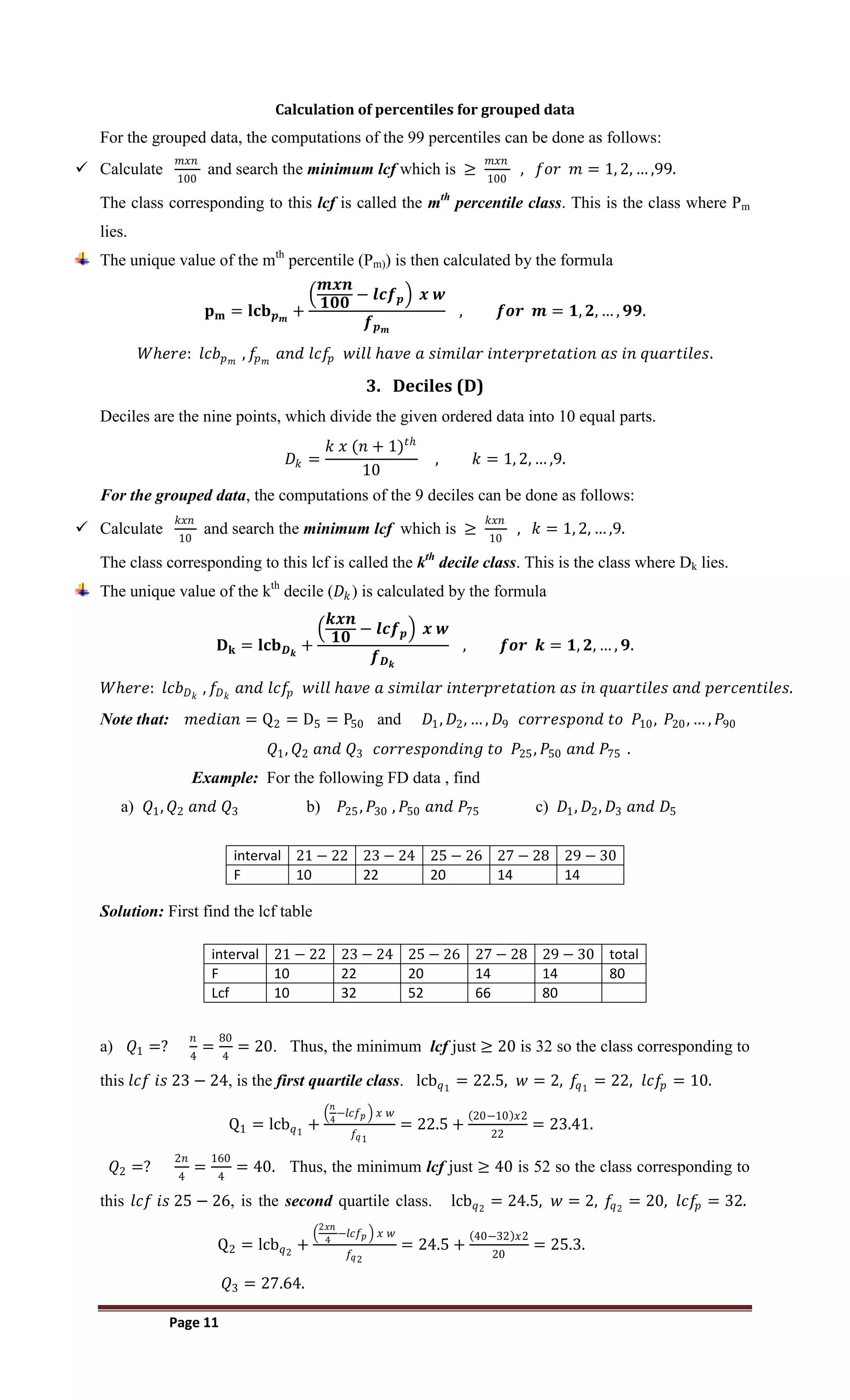
SlideShare a Scribd company logo
Page 1
CHAPTER - 2
2. Summarization of Data
2.1 Measures of Central Tendency
The most important objective of a statistical analysis is to determine a single value for the entire
mass of data, which describes the overall level of the group of observations and can be called a
representative of the whole set of data. It tells us where the center of the distribution of data is
located. The most commonly used measures of central tendencies are :
 The Mean (Arithmetic mean, Weighted mean, Geometric mean and Harmonic means)
 The Mode
 The Median
The Summation Notation:
 Let 𝑋1, 𝑋2, … , 𝑋𝑁 be the number of measurements where 𝑁 is the total number of
observation and 𝑋𝑖, is the ith
observation.
 Very often in statistics an algebraic expression of the form 𝑋1 + 𝑋2 + ⋯ + 𝑋𝑁 is used in
a formula to compute a statistic. It is tedious to write an expression like this very often,
so mathematicians have developed a shorthand notation to represent a sum of scores,
called the summation notation.
 The symbol 𝑋𝑖
𝑁
𝑖=1 is a mathematical shorthand for 𝑋1 + 𝑋2 + ⋯ + 𝑋𝑁.
𝑇𝑕𝑒𝑟𝑒𝑓𝑜𝑟𝑒, 𝑿𝒊
𝑵
𝒊=𝟏 = 𝑿𝟏 + 𝑿𝟐 + ⋯ + 𝑿𝑵 → 𝑓𝑜𝑟 𝑡𝑕𝑒 𝑝𝑜𝑝𝑢𝑙𝑎𝑡𝑖𝑜𝑛𝑠.
𝑿𝒊
𝒏
𝒊=𝟏 = 𝑿𝟏 + 𝑿𝟐 + ⋯ + 𝑿𝒏 → 𝑓𝑜𝑟 𝑡𝑕𝑒 𝑠𝑎𝑚𝑝𝑙𝑒𝑠.
Example: Suppose the following were scores (marks) made on the first assignment for
five students in the class: 5, 7, 7, 6, 𝑎𝑛𝑑 8. Write their marks using summation notation.
Solution: 𝑋𝑖
5
𝑖=1 = 𝑋1 + 𝑋2 + ⋯ + 𝑋5 = 5 + 7 + 7 + 6 + 8 = 33
Properties of summation
1. 𝑐
𝑛
𝑖=1 = 𝑛𝑐 𝑓𝑜𝑟 𝑎𝑛𝑦 𝑐𝑜𝑛𝑠𝑡𝑎𝑛𝑡 𝑐.
2. 𝑐𝑋𝑖
𝑛
𝑖=1 = 𝑐 𝑋𝑖
𝑛
𝑖=1
3. (𝑋𝑖 ± 𝑐)
𝑛
𝑖=1 = 𝑋𝑖
𝑛
𝑖=1 ± 𝑛𝑐
4. (𝑌𝑖+𝑋𝑖)
𝑛
𝑖=1 = 𝑋𝑖
𝑛
𝑖=1 + 𝑌𝑖
𝑛
𝑖=1
5. 𝑋𝑖𝑌𝑖
𝑛
𝑖=1 = 𝑋1𝑌1 + 𝑋2𝑌2 + ⋯ + 𝑋𝑛𝑌𝑛
6. 1 + 2 + 3 + 4 + ⋯ + 𝑛 =
𝑛(𝑛+1)
2
7. 12
+ 22
+32
+ ⋯ + 𝑛2
=
𝑛 𝑛+1 (2𝑛+1)
6
2.2 Types of Measure of Central Tendency
2.2.1 The Mean
2.2.1.1 Arithmetic mean
The arithmetic mean of a sample is the sum of all observations divided by the number of
observations in the sample. i.e.
𝑺𝒂𝒎𝒑𝒍𝒆 𝒎𝒆𝒂𝒏 𝒐𝒓 𝒂𝒓𝒊𝒕𝒉𝒎𝒆𝒕𝒊𝒄 𝒎𝒆𝒂𝒏 =
𝒕𝒉𝒆 𝒔𝒖𝒎 𝒐𝒇 𝒂𝒍𝒍 𝒗𝒂𝒍𝒖𝒆𝒔 𝒊𝒏 𝒕𝒉𝒆 𝒔𝒂𝒎𝒑𝒍𝒆
𝒏𝒖𝒎𝒃𝒆𝒓 𝒐𝒇 𝒗𝒂𝒍𝒖𝒆𝒔 𝒊𝒏 𝒕𝒉𝒆 𝒔𝒂𝒎𝒑𝒍𝒆
Suppose that 𝑥1, 𝑥2, … , 𝑥𝑛 are n observed values in a sample of size n taken from a population
of size N. Then the arithmetic mean of the sample, denoted by 𝑥, is given by
Page 2
𝑿 =
𝑿𝟏+𝑿𝟐+⋯+𝑿𝒏
𝐧
=
𝑿𝒊
𝒏
𝒊=𝟏
𝒏
→ 𝐟𝐨𝐫 𝐬𝐚𝐦𝐩𝐥𝐞𝐬.
If we take an entire population, the population mean denoted by µ is given by
µ =
𝑿𝟏+𝑿𝟐+⋯+𝑿𝑵
𝐍
=
𝑿𝒊
𝑵
𝒊=𝟏
𝑵
→ 𝐟𝐨𝐫 𝐩𝐨𝐩𝐮𝐥𝐚𝐭𝐢𝐨𝐧𝐬.
In general, the sample arithmetic mean is calculated by
𝑿 =
𝑿𝒊
𝒏
𝒏
𝒊=𝟏 → 𝑓𝑜𝑟 𝑟𝑎𝑤 𝑑𝑡𝑎𝑡𝑎
𝒇𝒊𝑿𝒊
𝒇𝒊
𝒌
𝒊=𝟏 → 𝑓𝑜𝑟 𝑢𝑛𝑔𝑟𝑜𝑢𝑝𝑒𝑑 𝑑𝑎𝑡𝑎 𝑤𝑕𝑒𝑟𝑒 𝑓𝑖 = 𝑛.
𝑴𝒊𝑿𝒊
𝒇𝒊
𝒌
𝒊=𝟏 → 𝑓𝑜𝑟 𝑔𝑟𝑜𝑢𝑝𝑒𝑑 𝑑𝑎𝑡𝑎 𝑤𝑕𝑒𝑟𝑒 𝑓𝑖 = 𝑛.
Example 1: The net weights of five perfume bottles selected at random from the production
line 𝑎𝑟𝑒 85.4, 85.3, 84.9, 85.4 𝑎𝑛𝑑 85. What is the arithmetic mean weight of the sample
observation?
Solution; 𝐺𝑖𝑣𝑒𝑛 𝑛 = 5 𝑥1 = 85.4, 𝑥2 = 85.3, 𝑥3 = 84.9, 𝑥4 = 85.4 𝑎𝑛𝑑 𝑥5 = 85.
𝑋 =
𝑋𝑖
𝑛
𝑖=1
𝑛
=
85.4+85.3+84.9+85.4+ 85
5
=
426.6
5
= 85.32.
Example 2: Calculate the mean of the marks of 46 students given below;
Marks (𝑋𝑖) 9 10 11 12 13 14 15 16 17 18
Frequency (𝑓𝑖) 1 2 3 6 10 11 7 3 2 1
Solution: 𝑓𝑖 = 𝑛 = 46 is the sum of the frequencies or total number of observations.
To calculate 𝒇𝒊𝑿𝒊
𝑘
𝑖=1 consider the following table.
𝑋𝑖 9 10 11 12 13 14 15 16 17 18 Total
𝑓𝑖 1 2 3 6 10 11 7 3 2 1 46
𝒇𝒊𝑿𝒊 9 20 33 72 130 154 105 48 34 18 623
So 𝑋 =
𝒇𝒊𝑿𝒊
𝒇𝒊
𝒌
𝒊=𝟏 =
623
46
= 13.54.
Example 3: The net income of a sample of large importers of Urea was organized into the
following table. What is the arithmetic mean of net income?
Net income 2-4 5-7 8-10 11-13 14-16
Number of importers 1 4 10 3 2
Solution: 𝑓𝑖 = 𝑛 = 20 is the sum of the frequencies or total number of observations.
To calculate 𝒇𝒊𝒎𝒊
𝑘
𝑖=1 consider the following table.
Net income (CI) 2-4 5-7 8-10 11-13 14-16 Total
Number of importers (𝑓𝑖) 1 4 10 3 2 20
Class marks (𝑚𝑖) 3 6 9 12 15
𝒇𝒊𝒎𝒊 3 24 90 36 30 183
So 𝑋 =
𝒇𝒊𝒎𝒊
𝒇𝒊
𝒌
𝒊=𝟏 =
𝟏𝟖𝟑
𝟐𝟎
= 𝟗. 𝟏𝟓.
Example 4: From the following data, calculate the missing frequency? The mean number of
tablets to cure ever was 29.18.
Number of tablets 19 − 21 22 − 24 25 − 27 28 − 30 31 − 33 34 − 36 37 − 39
Number of persons cured 6 13 19 𝑓4 18 12 9
Page 3
Solution; 𝑓𝑖 = 𝑛 = 77 + 𝑓
4 is the sum of the frequencies or total number of observations.
To calculate 𝒇𝒊𝒎𝒊
𝑘
𝑖=1 consider the following table.
CI 19 − 21 22 − 24 25 − 27 28 − 30 31 − 33 34 − 36 37 − 39 Total
𝒇𝒊 6 13 19 𝑓4 18 12 9 77+𝑓
4
𝒎𝒊 20 23 26 29 32 35 38
𝒇𝒊𝒎𝒊 120 299 494 29𝑓4 576 420 342 2251 + 29𝑓4
𝑆𝑖𝑛𝑐𝑒 𝑚𝑒𝑎𝑛 𝑖𝑠 𝑔𝑖𝑣𝑒𝑛 𝑡𝑜 𝑏𝑒 29.18 𝑤𝑒 𝑕𝑎𝑣𝑒
𝑋 =
𝑓𝑖𝑚𝑖
𝑓𝑖
𝑘
𝑖=1
=≫ 29.18 =
2251 + 29𝑓
4
77+𝑓
4
=≫ 29.18 77+𝑓
4 = 2251 + 29𝑓
4
=≫ 29.18𝑓
4 − 29𝑓4 = 2251 − 2246.86 =≫ 0.18𝑓
4 = 4.14 =≫ 𝑓
4 =
4.14
0.18
= 23.
Combined mean
If we have an arithmetic means 𝑋1, 𝑋2, … , 𝑋𝑛 of n groups having the same unit of measurement
of a variable, with sizes 𝑛1, 𝑛2, … , 𝑛𝑛 observations respectively, we can compute the combined
mean of the variant values of the groups taken together from the individual means by
𝑿𝒄𝒐𝒎 =
𝒏𝟏𝒙𝟏+𝒏𝟐𝒙𝟐+⋯+𝒏𝒏𝒙𝒏
𝒏𝟏+𝒏𝟐+⋯+𝒏𝒏
=
𝒏𝒊𝒙𝒊
𝒏
𝒊=𝟏
𝒏𝒊
𝒏
𝒊=𝟏
Example 1: Compute the combined mean for the following two sets.
𝑺𝒆𝒕 𝑨: 1, 4, 12, 2, 8 𝑎𝑛𝑑 6 ; 𝑺𝒆𝒕 𝑩: 3, 6, 2, 7 𝑎𝑛𝑑 4.
Solution: 𝑛1 = 6, 𝑥1 =
𝑋𝑖
6
𝑖=1
𝒏𝟏
=
33
6
= 5.5 ; 𝑛2 = 6, 𝑥2 =
𝑋𝑖
5
𝑖=1
𝒏𝟐
=
22
5
= 4.4.
𝑋𝑐𝑜𝑚 =
𝑛1𝑥1 + 𝑛2𝑥2
𝑛1 + 𝑛2
=
6 𝑥 5.5 + 5 𝑥 4.4
6 + 5
=
55
11
= 5.
Example 2: The mean weight of 150 students in a certain class is 60 kg. The mean
weight of boys in the class is 70 kg and that of girl’s is 55 kg . Find the number of boys
and girls in the class?
Solution; Let 𝑛1 be the number of boys and 𝑛2 be the number of girls in the class.
Also let 𝑥1 , 𝑥2 𝑎𝑛𝑑 𝑥𝑐𝑜𝑚 be the mean weights of boys, girls and the mean weights of all
students respectively. Then 𝑥1 = 70, 𝑥2 = 55 𝑎𝑛𝑑 𝑥𝑐𝑜𝑚 = 60. 𝐶𝑙𝑒𝑎𝑟𝑙𝑦 𝑛1 + 𝑛2 = 150.
𝑋𝑐𝑜𝑚 =
𝑛1𝑥1+𝑛2𝑥2
𝑛1+𝑛2
=≫ 60 =
70 𝑛1+55𝑛2
𝑛1+𝑛2
=≫ 60 =
70 𝑛1+55𝑛2
150
=≫ 9000 = 70 𝑛1 + 55𝑛2 … . … 1 𝑎𝑛𝑑
150 = 𝑛1 + 𝑛2 … … (2)
𝑆𝑜𝑙𝑣𝑖𝑛𝑔 𝑒𝑞𝑢𝑎𝑡𝑖𝑜𝑛 (1) 𝑎𝑛𝑑 (2) 𝑠𝑖𝑚𝑢𝑙𝑡𝑎𝑛𝑒𝑜𝑢𝑠𝑙𝑦, 𝑤𝑒 𝑔𝑒𝑡 𝑛1 = 50 𝑎𝑛𝑑 𝑛2 = 100.
Disadvantages of the arithmetic mean
1. The mean is meaningless in the case of nominal or qualitative data.
2. In case of grouped data, if any class interval is open ended, arithmetic mean cannot be
calculated, since the class mark of this interval cannot be found.
2.2.1.2 Weighted mean
In the computation of arithmetic mean, we had given an equal importance to each observation.
Sometimes the individual values in the data may not have an equally importance. When this is
the case, we assigned to each weight which is proportional to its relative importance.
 The weighted mean of a set of values 𝑥1, 𝑥2, … , 𝑥𝑛 with corresponding weights
𝑤1, 𝑤2, … , 𝑤𝑛 denoted by 𝑥𝑤 is computed by:
Page 4
𝑿𝒘 =
𝒘𝟏𝒙𝟏 + 𝒘𝟐𝒙𝟐 + ⋯ + 𝒘𝒏𝒙𝒏
𝒘𝟏 + 𝒘𝟐 + ⋯ + 𝒘𝒏
=
𝒘𝒊𝒙𝒊
𝒏
𝒊=𝟏
𝒘𝒊
𝒏
𝒊=𝟏
The calculation of cumulative grade point average (CGPA) in Colleges and Universities is a
good example of weighted mean.
Example: If a student scores "A" in a 3 EtCTS course, "B" in a 6 EtCTS course, "B" in
another 5 EtCTS course and "D" in a 2 EtCTS course. Compute his /her GPA for the semester.
Solution: Here the numerical values of the letter grades are the values (i.e. 𝐴 = 4, 𝐵 =
3, 𝐶 = 2 𝑎𝑛𝑑 𝐷 = 1) and the corresponding EtCTS of the course are their respective
weights. i.e.
Grade values (𝒙𝒊) 4 3 3 1
Weight (𝒘𝒊) 3 6 5 2
𝑮𝑷𝑨 = 𝑿𝒘 =
𝒘𝟏𝒙𝟏+𝒘𝟐𝒙𝟐+⋯+𝒘𝒏𝒙𝒏
𝒘𝟏+𝒘𝟐+⋯+𝒘𝒏
=
𝒘𝒊𝒙𝒊
𝟒
𝒊=𝟏
𝒘𝒊
𝟒
𝒊=𝟏
=
4x3+3x6+3x5+1x2
3+6+5+2
=
12+18+15+2
16
=
47
16
= 2.9375.
2.2.1.3 Geometric mean
In algebra geometric mean is calculated in the case of geometric progression, but in statistics we
need not bother about the progression, here it is particular type of data for which the geometric
mean is of great importance because it gives a good mean value. If the observed values are
measured as ratios, proportions or percentages, then the geometric mean gives a better measure
of central tendency than any other means.
 The Geometrical mean of a set of values 𝑥1, 𝑥2, … , 𝑥𝑛 of n positive values is defined as the
nth
root of their product . That is,
𝐺. 𝑀 = 𝑥1 ∗ 𝑥2 ∗ … ∗ 𝑥𝑛
𝑛
Example: The G.M of 4, 8 and 6 is
𝐺. 𝑀 = 4 𝑥 8 𝑥 6
3
= 192
3
= 5.77.
In general, the sample geometric mean is calculated by
𝑮. 𝒎 =
𝑥1 ∗ 𝑥2 ∗ … ∗ 𝑥𝑛
𝑛
→ 𝑓𝑜𝑟 𝑟𝑎𝑤 𝑑𝑡𝑎𝑡𝑎
𝑥1
𝑓1 ∗ 𝑥2
𝑓2 ∗, … ,∗ 𝑥𝑘
𝑓𝑘
𝑛
→ 𝑓𝑜𝑟 𝑢𝑛𝑔𝑟𝑜𝑢𝑝𝑒𝑑 𝑑𝑎𝑡𝑎 𝑤𝑕𝑒𝑟𝑒 𝑛 = 𝑓𝑖 .
𝑚1
𝑓1 ∗ 𝑚2
𝑓2 ∗. , … ,∗ 𝑚𝑘
𝑓𝑘
𝑛
→ 𝑓𝑜𝑟 𝑔𝑟𝑜𝑢𝑝𝑒𝑑 𝑑𝑎𝑡𝑎 𝑤𝑕𝑒𝑟𝑒 𝑛 = 𝑓𝑖 .
Example1: The man gets three annual raises in his salary. At the end of first year, he
gets an increase of 4%, at the end of the second year, he gets an increase of 6% and at the
end of the third year, he gets an increase of 9% of his salary. What is the average
percentage increase in the three periods?
Solution: 𝐺. 𝑀 = 1.04 ∗ 1.06 ∗ 1.09
3
= 1.0631 => 1.0631 − 1 = 0.0631.
𝑇𝑕𝑒𝑟𝑒𝑓𝑜𝑟𝑒, 𝑡𝑕𝑒 𝑎𝑣𝑒𝑟𝑎𝑔𝑒 𝑝𝑒𝑟𝑐𝑒𝑛𝑡𝑎𝑔𝑒 𝑖𝑛𝑐𝑟𝑒𝑎𝑠𝑒 𝑖𝑠 6.31%.
Example 2: Compute the Geometric mean of the following data.
Values 2 4 6 8 10
Frequency 1 2 2 2 1
Page 5
𝑺𝒐𝒍𝒖𝒕𝒊𝒐𝒏: 𝑔. 𝑚 = 21 ∗ 42 ∗ 62 ∗ 82 ∗ 101
8
= 2 ∗ 16 ∗ 36 ∗ 64 ∗ 100
8
= 737280
8
= 5.41.
Example 3: Suppose that the profits earned by a certain construction company in four projects
were 3%, 2%, 4% & 6% respectively. What is the Geometric mean profit?
𝑺𝒐𝒍𝒖𝒕𝒊𝒐𝒏: 𝑔. 𝑚 = 3 ∗ 2 ∗ 4 ∗ 6
4
= 144
4
= 3.46.
𝑇𝑕𝑒𝑟𝑒𝑓𝑜𝑟𝑒; 𝑡𝑕𝑒 𝑔𝑒𝑜𝑚𝑒𝑡𝑟𝑖𝑐 𝑚𝑒𝑎𝑛 𝑝𝑟𝑜𝑓𝑖𝑡 𝑖𝑠 3.46 𝑝𝑒𝑟𝑐𝑒𝑛𝑡.
2.2.1.4 Harmonic mean
Another important mean is the harmonic mean, which is suitable measure of central tendency
when the data pertains to speed, rates and price.
 Let 𝑥1, 𝑥2, … , 𝑥𝑛 be n variant values in a set of observations, then simple harmonic
mean is given by: 𝑺. 𝑯. 𝑴 =
𝐧
𝟏
𝐱𝟏
+
𝟏
𝐱𝟐
+⋯+
𝟏
𝐱𝐧
=
𝐧
𝟏
𝐱𝐢
𝐧
𝐢=𝟏
 Note: SHM is used for equal distances, equal costs and equal rates.
Example 1: A motorist travels for three days at a rate (speed) of 480 km/day. On the first day he
travels 10 hours at a rate of 48 km/h, on the second day 12 hours at a rate of 40 km/h, on the
third day 15 hours at a rate of 32 km/h. What is the average speed?
Solution: Since the distance covered by the motorist is equal (𝑖. 𝑒. 𝑠1 = 480, 𝑠2 = 480, 𝑠3 =
480), so we use SHM.
𝑆. 𝐻. 𝑀 =
3
1/48+1/40+1/32
= 38.92 so the required average speed = 38.92 𝑘𝑚/𝑕.
We can check this, by using the known formula for average speed in elementary physics.
Check; 𝐴𝑣𝑒𝑟𝑎𝑔𝑒 𝑠𝑝𝑒𝑒𝑑 𝑉
𝑎𝑣 =
total distance covered
total time taken
=
𝑆𝑇
𝑡𝑇
=
480km +480km +480km
10hr+12hr+15hr
=
1440km
37hr
= 38.42 𝑘𝑚/ h.
Example 2: A business man spent 20 Birr for milk at 40 cents per liter in Mizan-Aman town and
another 20 Birr at 60 cents per liter in Tepi town. What is the average price of milk at two towns.
Solution: Since the price on the two towns are equal (20 Birr), so we use SHM.
𝐴𝑣𝑒𝑟𝑎𝑔𝑒 𝑝𝑟𝑖𝑐𝑒 (𝑝𝑎𝑣 ) = 𝑆. 𝐻. 𝑀 =
2
1
40
+
1
60
= 48 𝑐𝑒𝑛𝑡𝑠/𝑙𝑖𝑡𝑒𝑟.
Weighted harmonic mean (WHM)
 WHM is used for different distance, different cost and different rate.
𝑊. 𝐻. 𝑀 =
𝑤𝑖
wi
xi
Example 1: A driver travel for 3 days. On the 1st
day he drives for 10h at a speed of 48 km/h, on
the 2nd
day for 12h at 45 km/h and on the 3rd day for 15h at 40 km/h. What is the average speed?
Solution: since the distance covered by the driver is not equal, so we use WHM by taking
the distance as weights (wi).
𝑣𝑎𝑣 = 𝑤. 𝑕. 𝑚 =
𝑤𝑖
wi
xi
=
(480 + 540 + 600)𝑘𝑚
480
40 +
540
45
+
600
40 𝑕𝑟
= 43.32 𝑘𝑚/𝑕𝑟.
Example 2: A business man spent 20 Birr for milk at rate of 40 cents per liter in Mizan-Aman
town and 25 Birr at a price of 50 cents per liter in Tepi town. What is the average price ?
Page 6
Solution: Since the price on the two towns are different , so we use WHM by taking the cost as
weights (wi).
𝑝𝑎𝑣 = 𝑤. 𝑕. 𝑚 =
𝑤𝑖
wi
xi
=
20 + 25 𝑏𝑖𝑟𝑟
20
40
+
25
50
𝑏𝑖𝑟𝑟 𝑙/𝑐
= 45 𝑐/𝑙.
 (Finally If all the observations are positive) 𝐴. 𝑀 ≥ 𝐺. 𝑀 ≥ 𝐻. 𝑀.
Corrected mean
𝒙𝒄𝒐𝒓𝒓 = 𝒙𝒘 +
𝒄 − 𝒘
𝒏
𝑤𝑕𝑒𝑟𝑒 𝑥𝑤 𝑖𝑠 𝑡𝑕𝑒 𝑤𝑟𝑜𝑛𝑔 𝑚𝑒𝑎𝑛
 𝒄 𝑖𝑠 𝑡𝑕𝑒 𝑠𝑢𝑚 𝑜𝑓 𝑐𝑜𝑟𝑟𝑒𝑐𝑡 𝑣𝑎𝑙𝑢𝑒𝑠 𝑎𝑛𝑑 𝒘 𝑖𝑠 𝑡𝑕𝑒 𝑠𝑢𝑚 𝑜𝑓 𝑤𝑟𝑜𝑛𝑔 𝑣𝑎𝑙𝑢𝑒𝑠.
Example: The mean age of a group of 100 persons was found to be 32.02 years. Later on, it was
discovered that age of 57 was misread as 27. Find the corrected mean?
Solution: 𝑛 = 100, 𝑥𝑤 = 32.02 , 𝑐 = 57 𝑎𝑛𝑑 𝑤 = 27.
𝑥𝑐𝑜𝑟𝑟 = 𝑥𝑤 +
𝑐 − 𝑤
𝑛
= 32.02 +
57 − 27
100
= 32.02 + 0.3 = 32.32 𝑦𝑒𝑎𝑟𝑠.
Median and mode
2.2.2 The Median
Suppose we sort all the observations in numerical order, ranging from smallest to largest or vice
versa. Then the median is the middle value in the sorted list. We denote it by x.
Let 𝑥1, 𝑥2, … , 𝑥𝑛 be n ordered observations. Then the median is given by:
𝒙 =
𝑿 𝒏+𝟏
𝟐
𝐼𝑓 𝑛 𝑖𝑠 𝑜𝑑𝑑.
𝑿 𝒏
𝟐
+𝑿 𝒏
𝟐
+𝟏
𝟐
𝐼𝑓 𝑛 𝑖𝑠 𝑒𝑣𝑒𝑛.
Example 1: Find the median for the following data.
23, 16, 31, 77, 21, 14, 32, 6, 155, 9, 36, 24, 5, 27, 19
Solution: First arrange the given data in increasing order. That is
5, 6, 9, 14, 16, 19, 21, 23, 24, 27, 31, 32, 36, 77, 𝑎𝑛𝑑 155.
𝑛 = 15 =≫ 𝑜𝑑𝑑, 𝑥 = 𝑋 𝑛+1
2
= 𝑋 15+1
2
= 𝑋 8 = 23
Example 2: Find the median for the following data.
61, 62, 63, 64, 64, 60, 65, 61, 63, 64, 65, 66, 64, 63
Solution: First arrange the given data in increasing order. that is
60, 61, 61, 62, 63, 63, 63, 64, 64, 64, 65, 65 & 66.
𝑛 = 14 =≫ 𝑒𝑣𝑒𝑛, 𝑥 =
𝑋 𝑛
2
+ 𝑋 𝑛
2
+1
2
=
𝑋 14
2
+ 𝑋 14
2
+1
2
=
𝑋 7 + 𝑋 8
2
=
63 + 64
2
=
127
2
= 63.5
Median for ungrouped data
 Let 𝑥1, 𝑥2, … , 𝑥𝑘 have their corresponding frequencies 𝑓1, 𝑓2, … , 𝑓𝑘 then to find the median:
 First sort the data in ascending order.
 Construct the less than cumulative frequency (lcf) .
 If 𝑛 = fi
𝑘
𝑖=1 is odd, find
n+1
2
and search the smallest lcf which is ≥
n+1
2
. Then
the variant value corresponding to this lcf is the median.
 If n is even, find
n
2
&
𝑛
2
+ 1 and search the smallest lcf which is ≥
n
2
&
𝑛
2
+ 1 .
Then the average of the variant values corresponding to these lcf is the median.
Page 7
Example 1: Find the median for the following data.
Values (xi) 3 5 4 2 7 6
Frequency (fi) 2 1 3 2 1 1
Solution: First arrange the data in increasing order and construct the lcf table for this data.
Values (xi) 2 3 4 5 6 7
Frequency (fi) 2 2 3 1 1 1
Lcf 2 4 7 8 9 10
𝑛 = 10 =≫ 𝑒𝑣𝑒𝑛. 𝑆𝑜
𝑛
2
=
10
2
= 5 𝑎𝑛𝑑
𝑛
2
+ 1 =
10
2
+ 1 = 5 + 1 = 6.
Then the smallest LCF which is ≥ 5 & 6 𝑖𝑠 7 and the variant value corresponding to this LCF
is 4. Thus the median is x =
4+4
2
= 4.
Example 2: Calculate the median of the marks of 46 students given below.
Values (xi) 10 9 11 12 14 13 15 16 17 18
Frequency (fi) 2 1 3 6 10 11 7 3 2 1
Solution: First arrange the data in ascending order and construct the LCF table for this data.
Values (xi) 9 10 11 12 13 14 15 16 17 18
Frequency (fi) 1 2 3 6 11 10 7 3 2 1
LCF 1 3 6 12 23 33 40 43 45 46
𝑛 = 46 =≫ 𝑒𝑣𝑒𝑛. 𝑆𝑜
𝑛
2
=
46
2
= 23 𝑎𝑛𝑑
𝑛
2
+ 1 =
46
2
+ 1 = 23 + 1 = 24.
𝑇𝑕𝑒 𝑠𝑚𝑎𝑙𝑙𝑒𝑠𝑡 𝐿𝐶𝐹 ≥ 23 & 24 𝑎𝑟𝑒 23 & 33 𝑟𝑒𝑠𝑝𝑒𝑐𝑡𝑖𝑣𝑒𝑙𝑦 𝑎𝑛𝑑 the variant values
corresponding to these LCF are 13 & 14 respectively. Thus the median 𝑖𝑠 x =
13+14
2
= 13.5.
Median for grouped data
The formula for computing the median for grouped data is given by
𝒎𝒆𝒅𝒊𝒂𝒏 = 𝐱 = 𝐥𝐜𝐛𝒙 +
𝒏
𝟐
− 𝒍𝒄𝒇𝒑 𝒙 𝒘
𝒇𝒎
𝑊𝑕𝑒𝑟𝑒: 𝑙𝑐𝑏𝑥 − 𝑖𝑠 𝑡𝑕𝑒 𝒍𝒄𝒃 𝑜𝑓 𝑡𝑕𝑒 𝑚𝑒𝑑𝑖𝑎𝑛 𝑐𝑙𝑎𝑠𝑠.
 𝑛 − 𝑖𝑠 𝑡𝑕𝑒 𝑡𝑜𝑡𝑎𝑙 𝑛𝑢𝑚𝑏𝑒𝑟 𝑜𝑓 𝑜𝑏𝑠𝑒𝑟𝑣𝑎𝑡𝑖𝑜𝑛𝑠.
 𝑓𝑚 𝑖𝑠 𝑡𝑕𝑒 𝑓𝑟𝑒𝑞𝑢𝑒𝑛𝑐𝑦 𝑜𝑓 𝑡𝑕𝑒 𝑚𝑒𝑑𝑖𝑎𝑛 𝑐𝑙𝑎𝑠𝑠.
 𝑤 𝑖𝑠 𝑡𝑕𝑒 𝑤𝑖𝑑𝑡𝑕 𝑜𝑓 𝑡𝑕𝑒 𝑚𝑒𝑑𝑖𝑎𝑛 𝑐𝑙𝑎𝑠𝑠. 𝑟𝑒𝑐𝑎𝑙𝑙 ∶ 𝑤 = 𝑢𝑐𝑏 − 𝑙𝑐𝑏.
 𝑙𝑐𝑓𝑝 𝑖𝑠 𝑡𝑕𝑒 𝒍𝒄𝒇 𝑐𝑜𝑟𝑟𝑒𝑠𝑝𝑜𝑛𝑑𝑖𝑛𝑔 𝑡𝑜 𝑡𝑕𝑒 𝑐𝑙𝑎𝑠𝑠 𝒊𝒎𝒎𝒆𝒅𝒊𝒂𝒕𝒆𝒍𝒚 𝒑𝒓𝒆𝒄𝒆𝒅𝒊𝒏𝒈 𝑡𝑕𝑒 𝑚𝑒𝑑𝑖𝑎𝑛 𝑐𝑙𝑎𝑠𝑠.
 Note: The class corresponding to the smallest LCF which is ≥
n
2
is called the median
class. So that the median lies in this class.
Steps to calculate the median for grouped data
1. First construct the LCF table.
2. Determine the median class. To determine the median class, find
n
2
and search the
smallest LCF which is ≥
n
2
. Then the class corresponding to this lcf is the median
class.
Page 8
Example 1: Find the median for the following data.
Daily production 80 − 89 90 − 99 100 − 109 110 − 119 120 − 129 130 − 139
Frequency 5 9 20 8 6 2
Solution: First construct the LCF table.
Daily production(CI) 80 − 89 90 − 99 100 − 109 110 − 119 120 − 129 130 − 139
Frequency(fi) 5 9 20 8 6 2
Lcf 5 14 34 42 48 50
To obtain the median class , calculate
𝑛
2
=
50
2
= 25. Thus the smallest lcf which is ≥
𝑛
2
is 34. So
the class corresponding to this lcf is 100 − 109, 𝑖𝑠 𝑡𝑕𝑒 𝑚𝑒𝑑𝑖𝑎𝑛 𝑐𝑙𝑎𝑠𝑠.
𝑇𝑕𝑒𝑟𝑒𝑓𝑜𝑟𝑒, 𝑙𝑐𝑏𝑥 = 99.5, 𝑤 = 10, 𝑓
𝑚 = 20, 𝑙𝑐𝑓
𝑝 = 14.
𝑚𝑒𝑑𝑖𝑎𝑛 = x = lcb𝑥 +
𝑛
2
− 𝑙𝑐𝑓
𝑝 𝑥 𝑤
𝑓
𝑚
= 99.5 +
25 − 14 𝑥 10
20
= 105.
Properties of the median
1. The median is unique.
2. It can be computed for an open ended frequency distribution if the median does not lie in
an open ended class.
3. It is not affected by extremely large or small values .
4. It is not so suitable for algebraic manipulations.
5. It can be computed for ratio level, interval level and ordinal level data.
2.2.3 The mode
In every day speech, something is “in the mode” if it is fashionable or popular. In statistics this
“popularity” refers to frequency of observations.
Therefore, mode is the `most frequently observed value in a set of observations.
𝑬𝒙𝒂𝒎𝒑𝒍𝒆: 𝑺𝒆𝒕 𝑨: 10, 10, 9, 8, 5, 4, 5, 12, 10 𝑚𝑜𝑑𝑒 = 10 → 𝑢𝑛𝑖𝑚𝑜𝑑𝑎𝑙.
𝑺𝒆𝒕 𝑩: 10, 10, 9, 9, 8, 12, 15, 5 𝑚𝑜𝑑𝑒 = 9 &10 → 𝑏𝑖𝑚𝑜𝑑𝑎𝑙.
𝑺𝒆𝒕 𝑪: 4, 6, 7, 15, 12, 9 𝑛𝑜 𝑚𝑜𝑑𝑒.
Remark: In a set of observed values, all values occur once or equal number of times, there is no
mode. (See set C above).
Mode for a grouped data
If the data is grouped such that we are given frequency distribution of finite class intervals, we
do not know the value of every item, but we easily determine the class with highest frequency.
Therefore, the modal class is the class with the highest frequency. So that the mode of the
distribution lies in this class.
 To compute the mode for a grouped data we use the formula:
𝒎𝒐𝒅𝒆 = 𝑿 = 𝒍𝒄𝒃𝒙 +
∆𝟏
∆𝟏 + ∆𝟐
𝒙 𝒘
𝑤𝑕𝑒𝑟𝑒; ∆1= 𝑓
𝑚 − 𝑓
𝑝 , ∆2= 𝑓
𝑚 − 𝑓
𝑠
𝑊𝑕𝑒𝑟𝑒: 𝑙𝑐𝑏𝑥 – 𝑖𝑠 𝑡𝑕𝑒 𝒍𝒄𝒃 𝑜𝑓 𝑡𝑕𝑒 𝑚𝑜𝑑𝑎𝑙 𝑐𝑙𝑎𝑠𝑠.
𝑓𝑚 − 𝑖𝑠 𝑡𝑕𝑒 𝑓𝑟𝑒𝑞𝑢𝑒𝑛𝑐𝑦 𝑜𝑓 𝑡𝑕𝑒 𝑚𝑜𝑑𝑎𝑙 𝑐𝑙𝑎𝑠𝑠.
Page 9
𝑓𝑝 − 𝑖𝑠 𝑡𝑕𝑒 𝑓𝑟𝑒𝑞𝑢𝑒𝑛𝑐𝑦 𝑜𝑓 𝑡𝑕𝑒 𝑐𝑙𝑎𝑠𝑠 𝒑𝒓𝒆𝒄𝒆𝒅𝒊𝒏𝒈 𝑡𝑕𝑒 𝑚𝑜𝑑𝑎𝑙 𝑐𝑙𝑎𝑠𝑠.
𝑓
𝑠 − 𝑖𝑠 𝑡𝑕𝑒 𝑓𝑟𝑒𝑞𝑢𝑒𝑛𝑐𝑦 𝑜𝑓 𝑡𝑕𝑒 𝑐𝑙𝑎𝑠𝑠 𝒔𝒖𝒄𝒄𝒆𝒆𝒅𝒊𝒏𝒈 𝑡𝑕𝑒 𝑚𝑜𝑑𝑎𝑙 𝑐𝑙𝑎𝑠𝑠.
𝑤 − 𝑖𝑠 𝑡𝑕𝑒 𝑤𝑖𝑑𝑡𝑕 𝑜𝑓 𝑡𝑕𝑒 𝑚𝑜𝑑𝑎𝑙 𝑐𝑙𝑎𝑠𝑠.
Example 1: The ages of newly hired, unskilled employees are grouped into the following
distribution. Then compute the modal age?
Ages 18 − 20 21 − 23 24 − 26 27 − 29 30 − 32
Number 4 8 11 20 7
Solution: First we determine the modal class. The modal class is 27 − 29, since it has the highest
frequency. 𝑇𝑕𝑢𝑠, 𝑙𝑐𝑏𝑥 = 26.5, 𝑤 = 3, ∆1= 20 − 11 = 9, ∆2= 20 − 7 = 13.
𝑋 = 𝑙𝑐𝑏𝑥 +
∆1
∆1 + ∆2
𝑥 𝑤 = 26.5 +
9
9 + 13
𝑥 3 = 26.5 +
27
22
= 26.5 + 1.2 = 𝟐𝟕. 𝟕
Interpretation: The age of most of these newly hired employees is 27.7 (27 years and 7 months).
Example 2: The following table shows the distribution of a group of families according to their
expenditure per week. The median and the mode of the following distribution are known to be
25.50 Birr and 24.50 Birr respectively. Two frequency values are however missing from the
table. Find the missing frequencies.
Class interval 1 − 10 11 − 20 21 − 30 31 − 40 41 − 50
Frequency 14 𝑓2 27 𝑓4 15
Solution: The LCF table of the given distribution can be formed as follows.
Expenditure (CI) 1 − 10 11 − 20 21 − 30 31 − 40 41 − 50
Number of families (fi) 14 𝑓2 27 𝑓4 15
LCF 14 14 + 𝑓2 41 + 𝑓2 41 + 𝑓2 + 𝑓4 56 + 𝑓2 + 𝑓4
Here: 𝑛 = 56 + 𝑓2 + 𝑓4. Since the median and the mode are Birr 25.5 & 24.5 respectively then
the class 21 − 30 is the median class as well as the modal class.
25.5 = 20.5 +
56+𝑓2+𝑓4
2
−(14+𝑓2) x 10
27
(𝑖)
24.5 = 20.5 +
27−𝑓2 x 10
(27−𝑓2)+(27−𝑓4)
(𝑖𝑖)
𝐸𝑞𝑛. (𝑖) 𝑎𝑛𝑑 𝑒𝑞𝑛. (𝑖𝑖) 𝑐𝑎𝑛 𝑏𝑒 𝑤𝑟𝑖𝑡𝑡𝑒𝑛 𝑎𝑠
5 =
5 x 56+𝑓2+𝑓4 −10 x (14+𝑓2)
27
& 4 =
27−𝑓2 x 10
54−𝑓2−𝑓4
Further simplifying the above we get
𝑓2 − 𝑓4 = 1. (𝑖𝑖𝑖) &
3𝑓2
− 2𝑓4
= 27. (𝑖𝑣)
𝑆𝑜𝑙𝑣𝑖𝑛𝑔 𝑖𝑖𝑖 & 𝐼𝑉 , 𝑤𝑒 𝑔𝑒𝑡 𝑡𝑕𝑒 𝑣𝑎𝑙𝑢𝑒𝑠 𝑜𝑓 𝑓2
& 𝑓4
𝑎𝑠 𝑓2
= 25 & 𝑓4
= 24.
Properties of mode
1. it is not affected by extreme values.
2. It can be calculated for distribution with open ended classes.
3. It can be computed for all levels of data i.e. nominal, ordinal, interval and ratio.
Page 10
4. The main drawback of mode is that often it does not exist.
5. Often its values are not unique.
2.3 Measure of non - central location (Quintiles’)
There are three types of quintiles. These are:
1. Quartiles
The quartiles are the three points, which divide a given order data into four equal parts. These
𝑄𝑖 =
𝑖 𝑥 (𝑛+1)𝑡𝑕
4
, 𝑖 = 1, 2, 3. → 𝑓𝑜𝑟 𝑟𝑎𝑤 𝑑𝑎𝑡𝑎.
Q1 is the value corresponding to (
n+1
4
)th
ordered observation.
Q2 is the value corresponding to 2 𝑥 (
n+1
4
)th
ordered observation.
Q3 is the value corresponding to 3 𝑥 (
n+1
4
)th
ordered observation.
Example: Consider the age data given below and calculate Q1, Q2, and Q3.
19, 20, 22, 22, 17, 22, 20, 23, 17, 18
Solution: First arrange the data in ascending order, n=10.
17, 17, 18, 19, 20, 20, 22, 22, 22, 23
Q1 = (
n+1
4
)th
= (
10+1
4
)th
= (2.75)th
observation = 2nd
observation + 0.75 (3rd
- 2nd
)
observation = 17 + 0.75(18 − 17) = 17.75
Therefore 25% of the observations are below 17.75
Q2 = 2𝑥(
n+1
4
)th
=2𝑥(
10+1
4
)th
= (5.5)th
observation = 5𝑡𝑕 + 0.5(6𝑡𝑕 − 5𝑡𝑕) = 20 +
0.5(20 − 20) = 20.
Q3 = 3𝑥(
n+1
4
)th
= 3𝑥(
10+1
4
)th
= (8.25)th
observation = 8th
+ 0.25x(9th
- 8th
) = 22+0.25x(22-
22)= 22
Calculation of quartiles for grouped data
 For the grouped data, the computations of the three quartiles can be done as follows:
 Calculate
𝑖𝑥𝑛
4
and search the minimum lcf which is ≥
𝑖𝑥𝑛
4
, 𝑓𝑜𝑟 𝑖 = 1, 2, 3.
The class corresponding to this lcf is called the ith
quartile class. This is the class where Qi lies.
The unique value of the ith
quartile (Qi) is then calculated by the formula
𝐐𝐢 = 𝐥𝐜𝐛𝒒𝒊
+
𝒊 𝒙 𝒏
𝟒
− 𝒍𝒄𝒇𝒑 𝒙 𝒘
𝒇𝒒𝒊
, 𝒇𝒐𝒓 𝒊 = 𝟏, 𝟐, 𝟑.
𝑊𝑕𝑒𝑟𝑒: lcb𝑞𝑖
− 𝑖𝑠 𝑡𝑕𝑒 𝒍𝒄𝒃 𝑜𝑓 𝑡𝑕𝑒 𝑖𝑡𝑕 𝑞𝑢𝑎𝑟𝑡𝑖𝑙𝑒 𝑐𝑙𝑎𝑠𝑠.
 𝑓𝑞𝑖
− 𝑖𝑠 𝑡𝑕𝑒 𝑓𝑟𝑒𝑞𝑢𝑒𝑛𝑐𝑦 𝑜𝑓 𝑡𝑕𝑒 𝑖𝑡𝑕 𝑞𝑢𝑎𝑟𝑡𝑖𝑙𝑒 𝑐𝑙𝑎𝑠𝑠.
 𝑙𝑐𝑓
𝑝 𝑖𝑠 𝑡𝑕𝑒 𝑙𝑐𝑓 𝑐𝑜𝑟𝑟𝑒𝑠𝑝𝑜𝑛𝑑𝑖𝑛𝑔 𝑡𝑜 𝑡𝑕𝑒 𝑐𝑙𝑎𝑠𝑠 𝒊𝒎𝒎𝒆𝒅𝒊𝒂𝒕𝒆𝒍𝒚 𝒑𝒓𝒆𝒄𝒆𝒅𝒊𝒏𝒈 𝑡𝑕𝑒 𝑖𝑡𝑕 𝑞𝑢𝑎𝑟𝑡𝑖𝑙𝑒 𝑐𝑙𝑎𝑠𝑠.
𝑁𝑜𝑡𝑒: 𝑄2 = 𝑚𝑒𝑑𝑖𝑎𝑛
2. Percentiles (P)
Percentiles are 99 points, which divide a given ordered data into 100 equal parts. These
𝑃
𝑚 =
𝑚 𝑥 (𝑛 + 1)𝑡𝑕
100
, 𝑚 = 1, 2, … ,99. → 𝑓𝑜𝑟 𝑟𝑎𝑤 𝑑𝑎𝑡𝑎.
Page 11
Calculation of percentiles for grouped data
For the grouped data, the computations of the 99 percentiles can be done as follows:
 Calculate
𝑚𝑥𝑛
100
and search the minimum lcf which is ≥
𝑚𝑥𝑛
100
, 𝑓𝑜𝑟 𝑚 = 1, 2, … ,99.
The class corresponding to this lcf is called the mth
percentile class. This is the class where Pm
lies.
The unique value of the mth
percentile (Pm)) is then calculated by the formula
𝐩𝐦 = 𝐥𝐜𝐛𝒑𝒎
+
𝒎𝒙𝒏
𝟏𝟎𝟎
− 𝒍𝒄𝒇𝒑 𝒙 𝒘
𝒇𝒑𝒎
, 𝒇𝒐𝒓 𝒎 = 𝟏, 𝟐, … , 𝟗𝟗.
𝑊𝑕𝑒𝑟𝑒: 𝑙𝑐𝑏𝑝𝑚
, 𝑓𝑝𝑚
𝑎𝑛𝑑 𝑙𝑐𝑓𝑝 𝑤𝑖𝑙𝑙 𝑕𝑎𝑣𝑒 𝑎 𝑠𝑖𝑚𝑖𝑙𝑎𝑟 𝑖𝑛𝑡𝑒𝑟𝑝𝑟𝑒𝑡𝑎𝑡𝑖𝑜𝑛 𝑎𝑠 𝑖𝑛 𝑞𝑢𝑎𝑟𝑡𝑖𝑙𝑒𝑠.
3. Deciles (D)
Deciles are the nine points, which divide the given ordered data into 10 equal parts.
𝐷𝑘 =
𝑘 𝑥 (𝑛 + 1)𝑡𝑕
10
, 𝑘 = 1, 2, … ,9.
For the grouped data, the computations of the 9 deciles can be done as follows:
 Calculate
𝑘𝑥𝑛
10
and search the minimum lcf which is ≥
𝑘𝑥𝑛
10
, 𝑘 = 1, 2, … ,9.
The class corresponding to this lcf is called the kth
decile class. This is the class where Dk lies.
The unique value of the kth
decile (𝐷𝑘) is calculated by the formula
𝐃𝐤 = 𝐥𝐜𝐛𝑫𝒌
+
𝒌𝒙𝒏
𝟏𝟎
− 𝒍𝒄𝒇𝒑 𝒙 𝒘
𝒇𝑫𝒌
, 𝒇𝒐𝒓 𝒌 = 𝟏, 𝟐, … , 𝟗.
𝑊𝑕𝑒𝑟𝑒: 𝑙𝑐𝑏𝐷𝑘
, 𝑓𝐷𝑘
𝑎𝑛𝑑 𝑙𝑐𝑓𝑝 𝑤𝑖𝑙𝑙 𝑕𝑎𝑣𝑒 𝑎 𝑠𝑖𝑚𝑖𝑙𝑎𝑟 𝑖𝑛𝑡𝑒𝑟𝑝𝑟𝑒𝑡𝑎𝑡𝑖𝑜𝑛 𝑎𝑠 𝑖𝑛 𝑞𝑢𝑎𝑟𝑡𝑖𝑙𝑒𝑠 𝑎𝑛𝑑 𝑝𝑒𝑟𝑐𝑒𝑛𝑡𝑖𝑙𝑒𝑠.
Note that: 𝑚𝑒𝑑𝑖𝑎𝑛 = Q2 = D5 = P50 and 𝐷1, 𝐷2, … , 𝐷9 𝑐𝑜𝑟𝑟𝑒𝑠𝑝𝑜𝑛𝑑 𝑡𝑜 𝑃10, 𝑃20, … , 𝑃90
𝑄1, 𝑄2 𝑎𝑛𝑑 𝑄3 𝑐𝑜𝑟𝑟𝑒𝑠𝑝𝑜𝑛𝑑𝑖𝑛𝑔 𝑡𝑜 𝑃25, 𝑃50 𝑎𝑛𝑑 𝑃75 .
Example: For the following FD data , find
a) 𝑄1, 𝑄2 𝑎𝑛𝑑 𝑄3 b) 𝑃25, 𝑃30 , 𝑃50 𝑎𝑛𝑑 𝑃75 c) 𝐷1, 𝐷2, 𝐷3 𝑎𝑛𝑑 𝐷5
interval 21 − 22 23 − 24 25 − 26 27 − 28 29 − 30
F 10 22 20 14 14
Solution: First find the lcf table
interval 21 − 22 23 − 24 25 − 26 27 − 28 29 − 30 total
F 10 22 20 14 14 80
Lcf 10 32 52 66 80
a) 𝑄1 =?
𝑛
4
=
80
4
= 20. Thus, the minimum lcf just ≥ 20 is 32 so the class corresponding to
this 𝑙𝑐𝑓 𝑖𝑠 23 − 24, is the first quartile class. lcb𝑞1
= 22.5, 𝑤 = 2, 𝑓
𝑞1
= 22, 𝑙𝑐𝑓
𝑝 = 10.
Q1 = lcb𝑞1
+
𝑛
4
−𝑙𝑐𝑓𝑝 𝑥 𝑤
𝑓𝑞1
= 22.5 +
20−10 𝑥2
22
= 23.41.
𝑄2 =?
2𝑛
4
=
160
4
= 40. Thus, the minimum lcf just ≥ 40 is 52 so the class corresponding to
this 𝑙𝑐𝑓 𝑖𝑠 25 − 26, is the second quartile class. lcb𝑞2
= 24.5, 𝑤 = 2, 𝑓
𝑞2
= 20, 𝑙𝑐𝑓
𝑝 = 32.
Q2 = lcb𝑞2
+
2𝑥𝑛
4
−𝑙𝑐𝑓𝑝 𝑥 𝑤
𝑓𝑞2
= 24.5 +
40−32 𝑥2
20
= 25.3.
𝑄3 = 27.64.
Page 12
b) 𝑃25 =?
25𝑥𝑛
100
=
25𝑥80
100
= 20. Thus, the minimum lcf just ≥ 20 is 32 so the class
corresponding to this 𝑙𝑐𝑓 𝑖𝑠 23 − 24, is the 25th
percentile class.
𝑇𝑕𝑢𝑠, lcb𝑝25
= 22.5, 𝑤 = 2, 𝑓
𝑝25
= 22, 𝑙𝑐𝑓
𝑝 = 10.
p25 = lcb𝑝25
+
25𝑥𝑛
100
− 𝑙𝑐𝑓
𝑝 𝑥 𝑤
𝑓
𝑝25
= 22.5 +
20 − 10 𝑥 2
22
= 23.41.
p20 = 23.045.
p30 = 23.77.
p50 = 25.3.
p75 = 27.64.
C) 𝐷1 =?
1𝑥𝑛
10
=
80
10
= 8. Thus, the minimum lcf just ≥ 8 is 10 so the class corresponding to
this 𝑙𝑐𝑓 𝑖𝑠 21 − 22, is the first decile class. 𝑇𝑕𝑢𝑠, lcb𝐷1
= 20.5, 𝑤 = 2, 𝑓𝐷1
= 10, 𝑙𝑐𝑓
𝑝 = 0.
D1 = lcb𝐷1
+
1𝑥𝑛
10
− 𝑙𝑐𝑓𝑝 𝑥 𝑤
𝑓𝐷1
= 20.5 +
8 − 0 𝑥 2
10
= 22.1 =≫ 𝑢𝑝𝑡𝑜 𝑐𝑙𝑎𝑠𝑠𝑏𝑜𝑢𝑛𝑑𝑎𝑟𝑦.
D2 = 23.045.
D3 = 23.77.
D5 = 25.3.
:. Q1 = P25 , Q2 = P50 and Q3 = P75 D1 = P10, D2 = P20, D3 = P30 and D5 = P50
and median = Q2 = D5 = P50
2.4. Measures of variation (dispersion)
Measures of central tendency locate the center of the distribution. But they do not tell how
individual observations are scattered on either side of the center. The spread of observations
around the center is known as dispersion or variability. In other words; the degree to which
numerical data tend to spread about an average value is called dispersion or variation of the data.
 Small dispersion indicates high uniformity of the observation while larger dispersion
indicates less uniformity.
Types of Measures of Dispersion
The most commonly used measures of dispersions are:
1. The Range (R)
The Range is the difference b/n the highest and the smallest observation. That is;
𝑅 =
𝑋𝑚𝑎𝑥 − 𝑋𝑚𝑖𝑛 → 𝑓𝑜𝑟 𝑟𝑎𝑤 𝑎𝑛𝑑 𝑢𝑛𝑔𝑟𝑜𝑢𝑝𝑒𝑑 𝑑𝑎𝑡𝑎.
𝑈𝐶𝐿𝑙𝑎𝑠𝑡 − 𝐿𝐶𝐿𝑓𝑖𝑟𝑠𝑡 → 𝑓𝑜𝑟 𝑔𝑟𝑜𝑢𝑝𝑒𝑑 𝑑𝑎𝑡𝑎.
It is a quick and dirty measure of variability. Because of the range is greatly affected by extreme
values, it may give a distorted picture of the scores.
Range is a measure of absolute dispersion and as such cannot be used for comparing variability
of two distributions expressed in different units.
4. Variance and Standard Deviation
Variance: is the average of the squares of the deviations taken from the mean.
Suppose that 𝑥1, 𝑥2, … , 𝑥𝑁 be the set of observations on N populations. Then,
𝑃𝑜𝑝𝑢𝑙𝑎𝑡𝑖𝑜𝑛 𝑣𝑎𝑟𝑖𝑎𝑛𝑐𝑒 = 𝜎2
=
𝑥𝑖 − 𝜇 2
𝑁
𝑖=1
𝑁
=
𝑥𝑖
2 − 𝑁𝜇2
𝑁
𝑖=1
𝑁
. → 𝑓𝑜𝑟 𝑝𝑜𝑝𝑢𝑙𝑎𝑡𝑖𝑜𝑛.
𝑆𝑎𝑚𝑝𝑙𝑒 𝑣𝑎𝑟𝑖𝑎𝑛𝑐𝑒 = 𝑠2
=
𝑥𝑖 − 𝑥 2
𝑛
𝑖=1
𝑛−1
=
𝑥𝑖
2 − 𝑛𝑥2
𝑛
𝑖=1
𝑛−1
. → 𝑓𝑜𝑟 𝑠𝑎𝑚𝑝𝑙𝑒.
Page 13
In general, the sample variance is computed by:
𝑠2
=
𝑥𝑖 − 𝑥 2
𝑛
𝑖=1
𝑛 − 1
=
𝑥𝑖
2
− 𝑛𝑥2
𝑛
𝑖=1
𝑛 − 1
. → 𝑓𝑜𝑟 𝑟𝑎𝑤 𝑑𝑎𝑡𝑎.
𝑓𝑖 𝑥𝑖 − 𝑥 2
𝑘
𝑖=1
𝑓𝑖
𝑘
𝑖=1 − 1
=
𝑓𝑖𝑥𝑖
2
− 𝑛𝑥2
𝑘
𝑖=1
𝑛 − 1
. → 𝑓𝑜𝑟 𝑢𝑛𝑔𝑟𝑜𝑢𝑝𝑒𝑑 𝑑𝑎𝑡𝑎.
𝑓𝑖 𝑚𝑖 − 𝑥 2
𝑘
𝑖=1
𝑓𝑖
𝑘
𝑖=1 − 1
=
𝑓𝑖𝑚𝑖
2
− 𝑛𝑥2
𝑘
𝑖=1
𝑛 − 1
. → 𝑓𝑜𝑟 𝑔𝑟𝑜𝑢𝑝𝑒𝑑 𝑑𝑎𝑡𝑎.
Standard Deviation: it is the square root of variance. Its advantage over the variance is that it is
in the same units as the variable under the consideration. It is a measure of the average variation
in a set of data. It is a measure of how far, on the average, an individual measurements is from
the mean. 𝑆. 𝑑 = 𝑣𝑎𝑟𝑖𝑎𝑛𝑐𝑒 = 𝑆2 = 𝑆.
Example 1: Compute the variance for the sample: 5, 14, 2, 2 and 17.
Solution: 𝑛 = 5 , 𝑥𝑖 = 40,
𝑛
𝑖=1 𝑥 = 8 , 𝑥𝑖
2
𝑛
𝑖=1 = 518 .
𝑠2
=
𝑥𝑖
2
− 𝑛𝑥2
𝑛
𝑖=1
𝑛 − 1
=
518 − 5 𝑥 82
5 − 1
= 49.5. , 𝑆 = 49.5 = 7.04.
Example 2: Suppose the data given below indicates time in minute required for a laboratory
experiment to compute a certain laboratory test. Calculate the mean, variance and standard
deviation for the following data.
𝒙𝒊 32 36 40 44 48 Total
𝒇𝒊 2 5 8 4 1 20
𝒇𝒊𝒙𝒊 64 180 320 176 48 788
𝒇𝒊 𝒙𝒊
𝟐 2048 6480 12800 7744 2304 31376
𝑥 =
𝒇𝒊𝒙𝒊
𝑛
𝑖=1
𝑛
=
788
20
= 39.4 , 𝑠2
=
𝒇𝒊𝑥𝑖
2
− 𝑛𝑥2
𝑛
𝑖=1
𝑛−1
=
31376−20 𝑥 39.4 2
19
= 17.31. , 𝑆 = 17.31 = 4.16.
Properties of Variance
1. The variance is always non-negative ( 𝑠2
≥ 0).
2. If every element of the data is multiplied by a constant "c", then the new variance
𝑠2
𝑛𝑒𝑤 = 𝑐2
𝑥 𝑠2
𝑜𝑙𝑑 .
3. When a constant is added to all elements of the data, then the variance does not change.
4. The variance of a constant (c) measured in n times is zero. i.e. (var(c) = 0).
Exercise: Verify the above properties.
Uses of the Variance and Standard Deviation
1. They can be used to determine the spread of the data. If the variance or S.D is large, then
the data are more dispersed.
2. They are used to measure the consistency of a variable.
3. They are used quit often in inferential statistics.
5. Coefficient of Variation (C.V)
Whenever the two groups have the same units of measurement, the variance and S.D for each
can be compared directly. A statistics that allows one to compare two groups when the units of
measurement are different is called coefficient of variation. It is computed by:
𝐶. 𝑉 =
𝜎
𝜇
𝑥 100% → 𝑓𝑜𝑟 𝑝𝑜𝑝𝑢𝑙𝑎𝑡𝑖𝑜𝑛.
𝐶. 𝑉 =
𝑆
𝑥
𝑥 100% → 𝑓𝑜𝑟 𝑠𝑎𝑚𝑝𝑙𝑒.
Page 14
Example: The following data refers to the hemoglobin level for 5 males and 5 female students.
In which case , the hemoglobin level has high variability (less consistency).
For males (xi) 13 13.8 14.6 15.6 17
For females (xi) 12 12.5 13.8 14.6 15.6
Solution: 𝑥𝑚𝑎𝑙𝑒 =
13+13.8+14.6+15.6+17
5
=
74
5
= 14.8 , 𝑥𝑓𝑒𝑚𝑎𝑙𝑒 =
12+12.5+13.8+14.6+15.6
5
=
68
5
= 13.7.
𝑠2
𝑚𝑎𝑙𝑒𝑠 =
𝑥𝑖
2 − 𝑛𝑥2
𝑛
𝑖=1
𝑛−1
= 2.44. , 𝑆𝑚𝑎𝑙𝑒𝑠 = 2.44 = 1.56205.,
𝑠2
𝑓𝑒𝑚𝑎𝑙𝑒𝑠 =
𝑥𝑖
2
− 𝑛𝑥2
𝑛
𝑖=1
𝑛 − 1
= 2.19. , 𝑆𝑓𝑒𝑚𝑎𝑙𝑒𝑠 = 2.19 = 1.479865.
𝐶. 𝑉𝑚𝑎𝑙𝑒𝑠 =
𝑆𝑚𝑎𝑙𝑒𝑠
𝑥𝑚𝑎𝑙𝑒
𝑥 100% =
1.56205
14.8
𝑥100% = 𝟏𝟎. 𝟓𝟔%,
𝐶. 𝑉𝑓𝑒𝑚𝑎𝑙𝑒𝑠 =
𝑆𝑓𝑒𝑚𝑎𝑙𝑒𝑠
𝑥𝑓𝑒𝑚𝑎𝑙𝑒
𝑥 100% =
1.479865
13.7
𝑥100% = 𝟏𝟎. 𝟖%.
Therefore, the variability in hemoglobin level is higher for females than for males.
6. Standard Scores (Z-Scores)
 It is used for describing the relative position of a single score in the entire set of data in
terms of the mean and standard deviation.
 It is used to compare two observations coming from different groups.
 If X is a measurement (an observation) from a distribution with mean 𝑥 and
standard deviation S, then its value in standard units is
𝑍 =
𝑋−𝜇
𝜎
→ 𝑓𝑜𝑟 𝑝𝑜𝑝𝑢𝑙𝑎𝑡𝑖𝑜𝑛.
𝑍 =
𝑥 − 𝑥
𝑆
→ 𝑓𝑜𝑟 𝑠𝑎𝑚𝑝𝑙𝑒.
 Z gives the number of standard deviation a particular observation lie above
or below the mean.
 A positive Z-score indicates that the observation is above the mean.
 A negative Z-score indicates that the observation is below the mean.
Example: Two sections were given an examination on a certain course. For section 1, the
average mark (score) was 72 with standard deviation of 6 and for section 2, the average mark
(score) was 85 with standard deviation of 7. If student A from section 1 scored 84 and student B
from section 2 scored 90, then who perform a better relative to the group?
Solution: 𝑍 𝑠𝑐𝑜𝑟𝑒 𝑓𝑜𝑟 𝐴 𝑖𝑠 𝑍 =
𝑥−𝑥
𝑆
=
84−72
6
= 2.
𝑍 𝑠𝑐𝑜𝑟𝑒 𝑓𝑜𝑟 𝐵 𝑖𝑠 𝑍 =
𝑥−𝑥
𝑆
=
90−85
7
= 0.71.
Since ZA > ZB i.e. 2 > 0.71, student A performed better relative to his group than student B.
Therefore, student A has performed better relative to his group because the score's of student A
is two standard deviation above the mean score of section 1 while the score of student B is only
0.71 standard deviation above the mean score of students in section 2.

More Related Content

What's hot

Nossi ch 11
Nossi ch 11Nossi ch 11
Nossi ch 11
lesaturner
 
Lecture on Measures of Variability/Dispersion by RDSII
Lecture on Measures of Variability/Dispersion by RDSIILecture on Measures of Variability/Dispersion by RDSII
Lecture on Measures of Variability/Dispersion by RDSII
REYNALDO II SALAYOG
 
Measures of central tendancy
Measures of central tendancy Measures of central tendancy
Measures of central tendancy
supriyamahesh
 
Mode
ModeMode
Solution to the Practice Test 3A, Normal Probability Distribution
Solution to the Practice Test 3A, Normal Probability DistributionSolution to the Practice Test 3A, Normal Probability Distribution
Solution to the Practice Test 3A, Normal Probability Distribution
Long Beach City College
 
Measures of central tendency
Measures of central tendencyMeasures of central tendency
Measures of central tendency
AashiPatel5
 
Measurement of central tendency
Measurement of central tendencyMeasurement of central tendency
Measurement of central tendency
BabatundeAdeyemi7
 
Real Applications of Normal Distributions
Real Applications of Normal Distributions Real Applications of Normal Distributions
Real Applications of Normal Distributions
Long Beach City College
 
Measures of Central Tendency
Measures of Central Tendency Measures of Central Tendency
Measures of Central Tendency
QUEENIE_
 
Lesson 23 planning data analyses using statistics
Lesson 23 planning data analyses using statisticsLesson 23 planning data analyses using statistics
Lesson 23 planning data analyses using statistics
mjlobetos
 
Measures of central tendency
Measures of central tendencyMeasures of central tendency
Measures of central tendency
Raj Teotia
 
Median
MedianMedian
Measures of central tendency and dispersion
Measures of central tendency and dispersionMeasures of central tendency and dispersion
Measures of central tendency and dispersion
Abhinav yadav
 
Measures of central tendency
Measures of central tendencyMeasures of central tendency
Measures of central tendency
gaya3lavanya92
 
Lesson 1 06 using the mean to measure central tendency
Lesson 1 06 using the mean to measure central tendency Lesson 1 06 using the mean to measure central tendency
Lesson 1 06 using the mean to measure central tendency
Perla Pelicano Corpez
 

What's hot (16)

Nossi ch 11
Nossi ch 11Nossi ch 11
Nossi ch 11
 
Lecture on Measures of Variability/Dispersion by RDSII
Lecture on Measures of Variability/Dispersion by RDSIILecture on Measures of Variability/Dispersion by RDSII
Lecture on Measures of Variability/Dispersion by RDSII
 
Measures of central tendancy
Measures of central tendancy Measures of central tendancy
Measures of central tendancy
 
Mode
ModeMode
Mode
 
Solution to the Practice Test 3A, Normal Probability Distribution
Solution to the Practice Test 3A, Normal Probability DistributionSolution to the Practice Test 3A, Normal Probability Distribution
Solution to the Practice Test 3A, Normal Probability Distribution
 
Measures of central tendency
Measures of central tendencyMeasures of central tendency
Measures of central tendency
 
Measurement of central tendency
Measurement of central tendencyMeasurement of central tendency
Measurement of central tendency
 
Real Applications of Normal Distributions
Real Applications of Normal Distributions Real Applications of Normal Distributions
Real Applications of Normal Distributions
 
Measures of Central Tendency
Measures of Central Tendency Measures of Central Tendency
Measures of Central Tendency
 
Lesson 23 planning data analyses using statistics
Lesson 23 planning data analyses using statisticsLesson 23 planning data analyses using statistics
Lesson 23 planning data analyses using statistics
 
Arithmetic mean
Arithmetic meanArithmetic mean
Arithmetic mean
 
Measures of central tendency
Measures of central tendencyMeasures of central tendency
Measures of central tendency
 
Median
MedianMedian
Median
 
Measures of central tendency and dispersion
Measures of central tendency and dispersionMeasures of central tendency and dispersion
Measures of central tendency and dispersion
 
Measures of central tendency
Measures of central tendencyMeasures of central tendency
Measures of central tendency
 
Lesson 1 06 using the mean to measure central tendency
Lesson 1 06 using the mean to measure central tendency Lesson 1 06 using the mean to measure central tendency
Lesson 1 06 using the mean to measure central tendency
 

Similar to CH2.pdf

Lesson plan in mathematics 9 (illustrations of quadratic equations)
Lesson plan in mathematics 9 (illustrations of quadratic equations)Lesson plan in mathematics 9 (illustrations of quadratic equations)
Lesson plan in mathematics 9 (illustrations of quadratic equations)
Decena15
 
Antiderivatives: Power, Sum and Difference
Antiderivatives: Power, Sum and DifferenceAntiderivatives: Power, Sum and Difference
Antiderivatives: Power, Sum and Difference
RivenBarquilla
 
Quantitative Aptitude - Average
Quantitative Aptitude - AverageQuantitative Aptitude - Average
Quantitative Aptitude - Average
Dr. Vaibhav Lowalekar
 
Mean median mode
Mean median modeMean median mode
Mean median mode
Abir Mridha
 
Lesson 7: Graphing Inequalities
Lesson 7: Graphing InequalitiesLesson 7: Graphing Inequalities
Lesson 7: Graphing Inequalities
Kevin Johnson
 
Comparative analysis of x^3+y^3=z^3 and x^2+y^2=z^2 in the Interconnected Sets
Comparative analysis of x^3+y^3=z^3 and x^2+y^2=z^2 in the Interconnected Sets Comparative analysis of x^3+y^3=z^3 and x^2+y^2=z^2 in the Interconnected Sets
Comparative analysis of x^3+y^3=z^3 and x^2+y^2=z^2 in the Interconnected Sets
Vladimir Godovalov
 
Equations.pptx
Equations.pptxEquations.pptx
Equations.pptx
JeralynAlabanzas2
 
Definite Integral 1.pptx
Definite Integral 1.pptxDefinite Integral 1.pptx
Definite Integral 1.pptx
RajiveGamer
 
MCA_UNIT-1_Computer Oriented Numerical Statistical Methods
MCA_UNIT-1_Computer Oriented Numerical Statistical MethodsMCA_UNIT-1_Computer Oriented Numerical Statistical Methods
MCA_UNIT-1_Computer Oriented Numerical Statistical Methods
Rai University
 
Summation-Notation-Jobelle-M-Quilana-Section-7001-1-1-B-Final (1).pptx
Summation-Notation-Jobelle-M-Quilana-Section-7001-1-1-B-Final (1).pptxSummation-Notation-Jobelle-M-Quilana-Section-7001-1-1-B-Final (1).pptx
Summation-Notation-Jobelle-M-Quilana-Section-7001-1-1-B-Final (1).pptx
jobelle15
 
Mean,Median and Mode Revision
Mean,Median and Mode Revision Mean,Median and Mode Revision
Mean,Median and Mode Revision
Puna Ripiye
 
Stochastic Optimization
Stochastic OptimizationStochastic Optimization
Stochastic Optimization
Mohammad Reza Jabbari
 
Lec
LecLec
A note on estimation of population mean in sample survey using auxiliary info...
A note on estimation of population mean in sample survey using auxiliary info...A note on estimation of population mean in sample survey using auxiliary info...
A note on estimation of population mean in sample survey using auxiliary info...
Alexander Decker
 
Presentation1.pptx
Presentation1.pptxPresentation1.pptx
Presentation1.pptx
Abebe334138
 
Arithmetic mean
Arithmetic meanArithmetic mean
Arithmetic mean
SoyaMathew1
 
Measures of spread revision
Measures of spread revision Measures of spread revision
Measures of spread revision
Puna Ripiye
 
Measures of Spread Revision
Measures of Spread Revision Measures of Spread Revision
Measures of Spread Revision
Puna Ripiye
 
Central Tendency.pptx
Central Tendency.pptxCentral Tendency.pptx
Central Tendency.pptx
CHIRANTANMONDAL2
 
Mean,median and mode revision card
Mean,median and mode revision cardMean,median and mode revision card
Mean,median and mode revision card
Puna Ripiye
 

Similar to CH2.pdf (20)

Lesson plan in mathematics 9 (illustrations of quadratic equations)
Lesson plan in mathematics 9 (illustrations of quadratic equations)Lesson plan in mathematics 9 (illustrations of quadratic equations)
Lesson plan in mathematics 9 (illustrations of quadratic equations)
 
Antiderivatives: Power, Sum and Difference
Antiderivatives: Power, Sum and DifferenceAntiderivatives: Power, Sum and Difference
Antiderivatives: Power, Sum and Difference
 
Quantitative Aptitude - Average
Quantitative Aptitude - AverageQuantitative Aptitude - Average
Quantitative Aptitude - Average
 
Mean median mode
Mean median modeMean median mode
Mean median mode
 
Lesson 7: Graphing Inequalities
Lesson 7: Graphing InequalitiesLesson 7: Graphing Inequalities
Lesson 7: Graphing Inequalities
 
Comparative analysis of x^3+y^3=z^3 and x^2+y^2=z^2 in the Interconnected Sets
Comparative analysis of x^3+y^3=z^3 and x^2+y^2=z^2 in the Interconnected Sets Comparative analysis of x^3+y^3=z^3 and x^2+y^2=z^2 in the Interconnected Sets
Comparative analysis of x^3+y^3=z^3 and x^2+y^2=z^2 in the Interconnected Sets
 
Equations.pptx
Equations.pptxEquations.pptx
Equations.pptx
 
Definite Integral 1.pptx
Definite Integral 1.pptxDefinite Integral 1.pptx
Definite Integral 1.pptx
 
MCA_UNIT-1_Computer Oriented Numerical Statistical Methods
MCA_UNIT-1_Computer Oriented Numerical Statistical MethodsMCA_UNIT-1_Computer Oriented Numerical Statistical Methods
MCA_UNIT-1_Computer Oriented Numerical Statistical Methods
 
Summation-Notation-Jobelle-M-Quilana-Section-7001-1-1-B-Final (1).pptx
Summation-Notation-Jobelle-M-Quilana-Section-7001-1-1-B-Final (1).pptxSummation-Notation-Jobelle-M-Quilana-Section-7001-1-1-B-Final (1).pptx
Summation-Notation-Jobelle-M-Quilana-Section-7001-1-1-B-Final (1).pptx
 
Mean,Median and Mode Revision
Mean,Median and Mode Revision Mean,Median and Mode Revision
Mean,Median and Mode Revision
 
Stochastic Optimization
Stochastic OptimizationStochastic Optimization
Stochastic Optimization
 
Lec
LecLec
Lec
 
A note on estimation of population mean in sample survey using auxiliary info...
A note on estimation of population mean in sample survey using auxiliary info...A note on estimation of population mean in sample survey using auxiliary info...
A note on estimation of population mean in sample survey using auxiliary info...
 
Presentation1.pptx
Presentation1.pptxPresentation1.pptx
Presentation1.pptx
 
Arithmetic mean
Arithmetic meanArithmetic mean
Arithmetic mean
 
Measures of spread revision
Measures of spread revision Measures of spread revision
Measures of spread revision
 
Measures of Spread Revision
Measures of Spread Revision Measures of Spread Revision
Measures of Spread Revision
 
Central Tendency.pptx
Central Tendency.pptxCentral Tendency.pptx
Central Tendency.pptx
 
Mean,median and mode revision card
Mean,median and mode revision cardMean,median and mode revision card
Mean,median and mode revision card
 

More from mekuannintdemeke

2.1. HRP.pdf
2.1. HRP.pdf2.1. HRP.pdf
2.1. HRP.pdf
mekuannintdemeke
 
COTM 4192 Chapter 2-2 Bituminous Materials.ppt
COTM 4192 Chapter 2-2 Bituminous Materials.pptCOTM 4192 Chapter 2-2 Bituminous Materials.ppt
COTM 4192 Chapter 2-2 Bituminous Materials.ppt
mekuannintdemeke
 
COTM 4192 Chapter 2-3 Stablized Pavement Materials.ppt
COTM 4192 Chapter 2-3 Stablized Pavement Materials.pptCOTM 4192 Chapter 2-3 Stablized Pavement Materials.ppt
COTM 4192 Chapter 2-3 Stablized Pavement Materials.ppt
mekuannintdemeke
 
COTM 4192 Chapter 2-2 Bituminous Materials.ppt
COTM 4192 Chapter 2-2 Bituminous Materials.pptCOTM 4192 Chapter 2-2 Bituminous Materials.ppt
COTM 4192 Chapter 2-2 Bituminous Materials.ppt
mekuannintdemeke
 
CE6503_Highway_Materials_Lec1_April21.pptx.pdf
CE6503_Highway_Materials_Lec1_April21.pptx.pdfCE6503_Highway_Materials_Lec1_April21.pptx.pdf
CE6503_Highway_Materials_Lec1_April21.pptx.pdf
mekuannintdemeke
 
COTM 4192 Chapter 2-3 Stablized Pavement Materials.pdf
COTM 4192 Chapter 2-3 Stablized Pavement Materials.pdfCOTM 4192 Chapter 2-3 Stablized Pavement Materials.pdf
COTM 4192 Chapter 2-3 Stablized Pavement Materials.pdf
mekuannintdemeke
 
Chapter One Procrument An Overview.pdf
Chapter One Procrument An Overview.pdfChapter One Procrument An Overview.pdf
Chapter One Procrument An Overview.pdf
mekuannintdemeke
 
Chapter -Two (3).pdf
Chapter -Two (3).pdfChapter -Two (3).pdf
Chapter -Two (3).pdf
mekuannintdemeke
 
Chapter -Two (2).pdf
Chapter -Two (2).pdfChapter -Two (2).pdf
Chapter -Two (2).pdf
mekuannintdemeke
 
CH1.pdf
CH1.pdfCH1.pdf
CH3.pdf
CH3.pdfCH3.pdf
CH6.pdf
CH6.pdfCH6.pdf
exercises.pdf
exercises.pdfexercises.pdf
exercises.pdf
mekuannintdemeke
 
Ch6
Ch6Ch6
Ch5
Ch5Ch5
Ch3
Ch3Ch3
Ch2
Ch2Ch2
Ch1
Ch1Ch1

More from mekuannintdemeke (18)

2.1. HRP.pdf
2.1. HRP.pdf2.1. HRP.pdf
2.1. HRP.pdf
 
COTM 4192 Chapter 2-2 Bituminous Materials.ppt
COTM 4192 Chapter 2-2 Bituminous Materials.pptCOTM 4192 Chapter 2-2 Bituminous Materials.ppt
COTM 4192 Chapter 2-2 Bituminous Materials.ppt
 
COTM 4192 Chapter 2-3 Stablized Pavement Materials.ppt
COTM 4192 Chapter 2-3 Stablized Pavement Materials.pptCOTM 4192 Chapter 2-3 Stablized Pavement Materials.ppt
COTM 4192 Chapter 2-3 Stablized Pavement Materials.ppt
 
COTM 4192 Chapter 2-2 Bituminous Materials.ppt
COTM 4192 Chapter 2-2 Bituminous Materials.pptCOTM 4192 Chapter 2-2 Bituminous Materials.ppt
COTM 4192 Chapter 2-2 Bituminous Materials.ppt
 
CE6503_Highway_Materials_Lec1_April21.pptx.pdf
CE6503_Highway_Materials_Lec1_April21.pptx.pdfCE6503_Highway_Materials_Lec1_April21.pptx.pdf
CE6503_Highway_Materials_Lec1_April21.pptx.pdf
 
COTM 4192 Chapter 2-3 Stablized Pavement Materials.pdf
COTM 4192 Chapter 2-3 Stablized Pavement Materials.pdfCOTM 4192 Chapter 2-3 Stablized Pavement Materials.pdf
COTM 4192 Chapter 2-3 Stablized Pavement Materials.pdf
 
Chapter One Procrument An Overview.pdf
Chapter One Procrument An Overview.pdfChapter One Procrument An Overview.pdf
Chapter One Procrument An Overview.pdf
 
Chapter -Two (3).pdf
Chapter -Two (3).pdfChapter -Two (3).pdf
Chapter -Two (3).pdf
 
Chapter -Two (2).pdf
Chapter -Two (2).pdfChapter -Two (2).pdf
Chapter -Two (2).pdf
 
CH1.pdf
CH1.pdfCH1.pdf
CH1.pdf
 
CH3.pdf
CH3.pdfCH3.pdf
CH3.pdf
 
CH6.pdf
CH6.pdfCH6.pdf
CH6.pdf
 
exercises.pdf
exercises.pdfexercises.pdf
exercises.pdf
 
Ch6
Ch6Ch6
Ch6
 
Ch5
Ch5Ch5
Ch5
 
Ch3
Ch3Ch3
Ch3
 
Ch2
Ch2Ch2
Ch2
 
Ch1
Ch1Ch1
Ch1
 

Recently uploaded

Characterization and the Kinetics of drying at the drying oven and with micro...
Characterization and the Kinetics of drying at the drying oven and with micro...Characterization and the Kinetics of drying at the drying oven and with micro...
Characterization and the Kinetics of drying at the drying oven and with micro...
Open Access Research Paper
 
AGRICULTURE Hydrophonic FERTILISER PPT.pptx
AGRICULTURE Hydrophonic FERTILISER PPT.pptxAGRICULTURE Hydrophonic FERTILISER PPT.pptx
AGRICULTURE Hydrophonic FERTILISER PPT.pptx
BanitaDsouza
 
Natural farming @ Dr. Siddhartha S. Jena.pptx
Natural farming @ Dr. Siddhartha S. Jena.pptxNatural farming @ Dr. Siddhartha S. Jena.pptx
Natural farming @ Dr. Siddhartha S. Jena.pptx
sidjena70
 
UNDERSTANDING WHAT GREEN WASHING IS!.pdf
UNDERSTANDING WHAT GREEN WASHING IS!.pdfUNDERSTANDING WHAT GREEN WASHING IS!.pdf
UNDERSTANDING WHAT GREEN WASHING IS!.pdf
JulietMogola
 
Summary of the Climate and Energy Policy of Australia
Summary of the Climate and Energy Policy of AustraliaSummary of the Climate and Energy Policy of Australia
Summary of the Climate and Energy Policy of Australia
yasmindemoraes1
 
growbilliontrees.com-Trees for Granddaughter (1).pdf
growbilliontrees.com-Trees for Granddaughter (1).pdfgrowbilliontrees.com-Trees for Granddaughter (1).pdf
growbilliontrees.com-Trees for Granddaughter (1).pdf
yadavakashagra
 
International+e-Commerce+Platform-www.cfye-commerce.shop
International+e-Commerce+Platform-www.cfye-commerce.shopInternational+e-Commerce+Platform-www.cfye-commerce.shop
International+e-Commerce+Platform-www.cfye-commerce.shop
laozhuseo02
 
Willie Nelson Net Worth: A Journey Through Music, Movies, and Business Ventures
Willie Nelson Net Worth: A Journey Through Music, Movies, and Business VenturesWillie Nelson Net Worth: A Journey Through Music, Movies, and Business Ventures
Willie Nelson Net Worth: A Journey Through Music, Movies, and Business Ventures
greendigital
 
Alert-driven Community-based Forest monitoring: A case of the Peruvian Amazon
Alert-driven Community-based Forest monitoring: A case of the Peruvian AmazonAlert-driven Community-based Forest monitoring: A case of the Peruvian Amazon
Alert-driven Community-based Forest monitoring: A case of the Peruvian Amazon
CIFOR-ICRAF
 
Artificial Reefs by Kuddle Life Foundation - May 2024
Artificial Reefs by Kuddle Life Foundation - May 2024Artificial Reefs by Kuddle Life Foundation - May 2024
Artificial Reefs by Kuddle Life Foundation - May 2024
punit537210
 
Celebrating World-environment-day-2024.pdf
Celebrating  World-environment-day-2024.pdfCelebrating  World-environment-day-2024.pdf
Celebrating World-environment-day-2024.pdf
rohankumarsinghrore1
 
Presentación Giulio Quaggiotto-Diálogo improbable .pptx.pdf
Presentación Giulio Quaggiotto-Diálogo improbable .pptx.pdfPresentación Giulio Quaggiotto-Diálogo improbable .pptx.pdf
Presentación Giulio Quaggiotto-Diálogo improbable .pptx.pdf
Innovation and Technology for Development Centre
 
Environmental Science Book By Dr. Y.K. Singh
Environmental Science Book By Dr. Y.K. SinghEnvironmental Science Book By Dr. Y.K. Singh
Environmental Science Book By Dr. Y.K. Singh
AhmadKhan917612
 
"Understanding the Carbon Cycle: Processes, Human Impacts, and Strategies for...
"Understanding the Carbon Cycle: Processes, Human Impacts, and Strategies for..."Understanding the Carbon Cycle: Processes, Human Impacts, and Strategies for...
"Understanding the Carbon Cycle: Processes, Human Impacts, and Strategies for...
MMariSelvam4
 
IPCC Vice Chair Ladislaus Change Central Asia Climate Change Conference 27 Ma...
IPCC Vice Chair Ladislaus Change Central Asia Climate Change Conference 27 Ma...IPCC Vice Chair Ladislaus Change Central Asia Climate Change Conference 27 Ma...
IPCC Vice Chair Ladislaus Change Central Asia Climate Change Conference 27 Ma...
ipcc-media
 
Bhopal Gas Leak Tragedy - A Night of death
Bhopal Gas Leak Tragedy - A Night of deathBhopal Gas Leak Tragedy - A Night of death
Bhopal Gas Leak Tragedy - A Night of death
upasana742003
 
NRW Board Paper - DRAFT NRW Recreation Strategy
NRW Board Paper - DRAFT NRW Recreation StrategyNRW Board Paper - DRAFT NRW Recreation Strategy
NRW Board Paper - DRAFT NRW Recreation Strategy
Robin Grant
 
Prevalence, biochemical and hematological study of diabetic patients
Prevalence, biochemical and hematological study of diabetic patientsPrevalence, biochemical and hematological study of diabetic patients
Prevalence, biochemical and hematological study of diabetic patients
Open Access Research Paper
 
DRAFT NRW Recreation Strategy - People and Nature thriving together
DRAFT NRW Recreation Strategy - People and Nature thriving togetherDRAFT NRW Recreation Strategy - People and Nature thriving together
DRAFT NRW Recreation Strategy - People and Nature thriving together
Robin Grant
 
ppt on beauty of the nature by Palak.pptx
ppt on  beauty of the nature by Palak.pptxppt on  beauty of the nature by Palak.pptx
ppt on beauty of the nature by Palak.pptx
RaniJaiswal16
 

Recently uploaded (20)

Characterization and the Kinetics of drying at the drying oven and with micro...
Characterization and the Kinetics of drying at the drying oven and with micro...Characterization and the Kinetics of drying at the drying oven and with micro...
Characterization and the Kinetics of drying at the drying oven and with micro...
 
AGRICULTURE Hydrophonic FERTILISER PPT.pptx
AGRICULTURE Hydrophonic FERTILISER PPT.pptxAGRICULTURE Hydrophonic FERTILISER PPT.pptx
AGRICULTURE Hydrophonic FERTILISER PPT.pptx
 
Natural farming @ Dr. Siddhartha S. Jena.pptx
Natural farming @ Dr. Siddhartha S. Jena.pptxNatural farming @ Dr. Siddhartha S. Jena.pptx
Natural farming @ Dr. Siddhartha S. Jena.pptx
 
UNDERSTANDING WHAT GREEN WASHING IS!.pdf
UNDERSTANDING WHAT GREEN WASHING IS!.pdfUNDERSTANDING WHAT GREEN WASHING IS!.pdf
UNDERSTANDING WHAT GREEN WASHING IS!.pdf
 
Summary of the Climate and Energy Policy of Australia
Summary of the Climate and Energy Policy of AustraliaSummary of the Climate and Energy Policy of Australia
Summary of the Climate and Energy Policy of Australia
 
growbilliontrees.com-Trees for Granddaughter (1).pdf
growbilliontrees.com-Trees for Granddaughter (1).pdfgrowbilliontrees.com-Trees for Granddaughter (1).pdf
growbilliontrees.com-Trees for Granddaughter (1).pdf
 
International+e-Commerce+Platform-www.cfye-commerce.shop
International+e-Commerce+Platform-www.cfye-commerce.shopInternational+e-Commerce+Platform-www.cfye-commerce.shop
International+e-Commerce+Platform-www.cfye-commerce.shop
 
Willie Nelson Net Worth: A Journey Through Music, Movies, and Business Ventures
Willie Nelson Net Worth: A Journey Through Music, Movies, and Business VenturesWillie Nelson Net Worth: A Journey Through Music, Movies, and Business Ventures
Willie Nelson Net Worth: A Journey Through Music, Movies, and Business Ventures
 
Alert-driven Community-based Forest monitoring: A case of the Peruvian Amazon
Alert-driven Community-based Forest monitoring: A case of the Peruvian AmazonAlert-driven Community-based Forest monitoring: A case of the Peruvian Amazon
Alert-driven Community-based Forest monitoring: A case of the Peruvian Amazon
 
Artificial Reefs by Kuddle Life Foundation - May 2024
Artificial Reefs by Kuddle Life Foundation - May 2024Artificial Reefs by Kuddle Life Foundation - May 2024
Artificial Reefs by Kuddle Life Foundation - May 2024
 
Celebrating World-environment-day-2024.pdf
Celebrating  World-environment-day-2024.pdfCelebrating  World-environment-day-2024.pdf
Celebrating World-environment-day-2024.pdf
 
Presentación Giulio Quaggiotto-Diálogo improbable .pptx.pdf
Presentación Giulio Quaggiotto-Diálogo improbable .pptx.pdfPresentación Giulio Quaggiotto-Diálogo improbable .pptx.pdf
Presentación Giulio Quaggiotto-Diálogo improbable .pptx.pdf
 
Environmental Science Book By Dr. Y.K. Singh
Environmental Science Book By Dr. Y.K. SinghEnvironmental Science Book By Dr. Y.K. Singh
Environmental Science Book By Dr. Y.K. Singh
 
"Understanding the Carbon Cycle: Processes, Human Impacts, and Strategies for...
"Understanding the Carbon Cycle: Processes, Human Impacts, and Strategies for..."Understanding the Carbon Cycle: Processes, Human Impacts, and Strategies for...
"Understanding the Carbon Cycle: Processes, Human Impacts, and Strategies for...
 
IPCC Vice Chair Ladislaus Change Central Asia Climate Change Conference 27 Ma...
IPCC Vice Chair Ladislaus Change Central Asia Climate Change Conference 27 Ma...IPCC Vice Chair Ladislaus Change Central Asia Climate Change Conference 27 Ma...
IPCC Vice Chair Ladislaus Change Central Asia Climate Change Conference 27 Ma...
 
Bhopal Gas Leak Tragedy - A Night of death
Bhopal Gas Leak Tragedy - A Night of deathBhopal Gas Leak Tragedy - A Night of death
Bhopal Gas Leak Tragedy - A Night of death
 
NRW Board Paper - DRAFT NRW Recreation Strategy
NRW Board Paper - DRAFT NRW Recreation StrategyNRW Board Paper - DRAFT NRW Recreation Strategy
NRW Board Paper - DRAFT NRW Recreation Strategy
 
Prevalence, biochemical and hematological study of diabetic patients
Prevalence, biochemical and hematological study of diabetic patientsPrevalence, biochemical and hematological study of diabetic patients
Prevalence, biochemical and hematological study of diabetic patients
 
DRAFT NRW Recreation Strategy - People and Nature thriving together
DRAFT NRW Recreation Strategy - People and Nature thriving togetherDRAFT NRW Recreation Strategy - People and Nature thriving together
DRAFT NRW Recreation Strategy - People and Nature thriving together
 
ppt on beauty of the nature by Palak.pptx
ppt on  beauty of the nature by Palak.pptxppt on  beauty of the nature by Palak.pptx
ppt on beauty of the nature by Palak.pptx
 

CH2.pdf

  • 1. Page 1 CHAPTER - 2 2. Summarization of Data 2.1 Measures of Central Tendency The most important objective of a statistical analysis is to determine a single value for the entire mass of data, which describes the overall level of the group of observations and can be called a representative of the whole set of data. It tells us where the center of the distribution of data is located. The most commonly used measures of central tendencies are :  The Mean (Arithmetic mean, Weighted mean, Geometric mean and Harmonic means)  The Mode  The Median The Summation Notation:  Let 𝑋1, 𝑋2, … , 𝑋𝑁 be the number of measurements where 𝑁 is the total number of observation and 𝑋𝑖, is the ith observation.  Very often in statistics an algebraic expression of the form 𝑋1 + 𝑋2 + ⋯ + 𝑋𝑁 is used in a formula to compute a statistic. It is tedious to write an expression like this very often, so mathematicians have developed a shorthand notation to represent a sum of scores, called the summation notation.  The symbol 𝑋𝑖 𝑁 𝑖=1 is a mathematical shorthand for 𝑋1 + 𝑋2 + ⋯ + 𝑋𝑁. 𝑇𝑕𝑒𝑟𝑒𝑓𝑜𝑟𝑒, 𝑿𝒊 𝑵 𝒊=𝟏 = 𝑿𝟏 + 𝑿𝟐 + ⋯ + 𝑿𝑵 → 𝑓𝑜𝑟 𝑡𝑕𝑒 𝑝𝑜𝑝𝑢𝑙𝑎𝑡𝑖𝑜𝑛𝑠. 𝑿𝒊 𝒏 𝒊=𝟏 = 𝑿𝟏 + 𝑿𝟐 + ⋯ + 𝑿𝒏 → 𝑓𝑜𝑟 𝑡𝑕𝑒 𝑠𝑎𝑚𝑝𝑙𝑒𝑠. Example: Suppose the following were scores (marks) made on the first assignment for five students in the class: 5, 7, 7, 6, 𝑎𝑛𝑑 8. Write their marks using summation notation. Solution: 𝑋𝑖 5 𝑖=1 = 𝑋1 + 𝑋2 + ⋯ + 𝑋5 = 5 + 7 + 7 + 6 + 8 = 33 Properties of summation 1. 𝑐 𝑛 𝑖=1 = 𝑛𝑐 𝑓𝑜𝑟 𝑎𝑛𝑦 𝑐𝑜𝑛𝑠𝑡𝑎𝑛𝑡 𝑐. 2. 𝑐𝑋𝑖 𝑛 𝑖=1 = 𝑐 𝑋𝑖 𝑛 𝑖=1 3. (𝑋𝑖 ± 𝑐) 𝑛 𝑖=1 = 𝑋𝑖 𝑛 𝑖=1 ± 𝑛𝑐 4. (𝑌𝑖+𝑋𝑖) 𝑛 𝑖=1 = 𝑋𝑖 𝑛 𝑖=1 + 𝑌𝑖 𝑛 𝑖=1 5. 𝑋𝑖𝑌𝑖 𝑛 𝑖=1 = 𝑋1𝑌1 + 𝑋2𝑌2 + ⋯ + 𝑋𝑛𝑌𝑛 6. 1 + 2 + 3 + 4 + ⋯ + 𝑛 = 𝑛(𝑛+1) 2 7. 12 + 22 +32 + ⋯ + 𝑛2 = 𝑛 𝑛+1 (2𝑛+1) 6 2.2 Types of Measure of Central Tendency 2.2.1 The Mean 2.2.1.1 Arithmetic mean The arithmetic mean of a sample is the sum of all observations divided by the number of observations in the sample. i.e. 𝑺𝒂𝒎𝒑𝒍𝒆 𝒎𝒆𝒂𝒏 𝒐𝒓 𝒂𝒓𝒊𝒕𝒉𝒎𝒆𝒕𝒊𝒄 𝒎𝒆𝒂𝒏 = 𝒕𝒉𝒆 𝒔𝒖𝒎 𝒐𝒇 𝒂𝒍𝒍 𝒗𝒂𝒍𝒖𝒆𝒔 𝒊𝒏 𝒕𝒉𝒆 𝒔𝒂𝒎𝒑𝒍𝒆 𝒏𝒖𝒎𝒃𝒆𝒓 𝒐𝒇 𝒗𝒂𝒍𝒖𝒆𝒔 𝒊𝒏 𝒕𝒉𝒆 𝒔𝒂𝒎𝒑𝒍𝒆 Suppose that 𝑥1, 𝑥2, … , 𝑥𝑛 are n observed values in a sample of size n taken from a population of size N. Then the arithmetic mean of the sample, denoted by 𝑥, is given by
  • 2. Page 2 𝑿 = 𝑿𝟏+𝑿𝟐+⋯+𝑿𝒏 𝐧 = 𝑿𝒊 𝒏 𝒊=𝟏 𝒏 → 𝐟𝐨𝐫 𝐬𝐚𝐦𝐩𝐥𝐞𝐬. If we take an entire population, the population mean denoted by µ is given by µ = 𝑿𝟏+𝑿𝟐+⋯+𝑿𝑵 𝐍 = 𝑿𝒊 𝑵 𝒊=𝟏 𝑵 → 𝐟𝐨𝐫 𝐩𝐨𝐩𝐮𝐥𝐚𝐭𝐢𝐨𝐧𝐬. In general, the sample arithmetic mean is calculated by 𝑿 = 𝑿𝒊 𝒏 𝒏 𝒊=𝟏 → 𝑓𝑜𝑟 𝑟𝑎𝑤 𝑑𝑡𝑎𝑡𝑎 𝒇𝒊𝑿𝒊 𝒇𝒊 𝒌 𝒊=𝟏 → 𝑓𝑜𝑟 𝑢𝑛𝑔𝑟𝑜𝑢𝑝𝑒𝑑 𝑑𝑎𝑡𝑎 𝑤𝑕𝑒𝑟𝑒 𝑓𝑖 = 𝑛. 𝑴𝒊𝑿𝒊 𝒇𝒊 𝒌 𝒊=𝟏 → 𝑓𝑜𝑟 𝑔𝑟𝑜𝑢𝑝𝑒𝑑 𝑑𝑎𝑡𝑎 𝑤𝑕𝑒𝑟𝑒 𝑓𝑖 = 𝑛. Example 1: The net weights of five perfume bottles selected at random from the production line 𝑎𝑟𝑒 85.4, 85.3, 84.9, 85.4 𝑎𝑛𝑑 85. What is the arithmetic mean weight of the sample observation? Solution; 𝐺𝑖𝑣𝑒𝑛 𝑛 = 5 𝑥1 = 85.4, 𝑥2 = 85.3, 𝑥3 = 84.9, 𝑥4 = 85.4 𝑎𝑛𝑑 𝑥5 = 85. 𝑋 = 𝑋𝑖 𝑛 𝑖=1 𝑛 = 85.4+85.3+84.9+85.4+ 85 5 = 426.6 5 = 85.32. Example 2: Calculate the mean of the marks of 46 students given below; Marks (𝑋𝑖) 9 10 11 12 13 14 15 16 17 18 Frequency (𝑓𝑖) 1 2 3 6 10 11 7 3 2 1 Solution: 𝑓𝑖 = 𝑛 = 46 is the sum of the frequencies or total number of observations. To calculate 𝒇𝒊𝑿𝒊 𝑘 𝑖=1 consider the following table. 𝑋𝑖 9 10 11 12 13 14 15 16 17 18 Total 𝑓𝑖 1 2 3 6 10 11 7 3 2 1 46 𝒇𝒊𝑿𝒊 9 20 33 72 130 154 105 48 34 18 623 So 𝑋 = 𝒇𝒊𝑿𝒊 𝒇𝒊 𝒌 𝒊=𝟏 = 623 46 = 13.54. Example 3: The net income of a sample of large importers of Urea was organized into the following table. What is the arithmetic mean of net income? Net income 2-4 5-7 8-10 11-13 14-16 Number of importers 1 4 10 3 2 Solution: 𝑓𝑖 = 𝑛 = 20 is the sum of the frequencies or total number of observations. To calculate 𝒇𝒊𝒎𝒊 𝑘 𝑖=1 consider the following table. Net income (CI) 2-4 5-7 8-10 11-13 14-16 Total Number of importers (𝑓𝑖) 1 4 10 3 2 20 Class marks (𝑚𝑖) 3 6 9 12 15 𝒇𝒊𝒎𝒊 3 24 90 36 30 183 So 𝑋 = 𝒇𝒊𝒎𝒊 𝒇𝒊 𝒌 𝒊=𝟏 = 𝟏𝟖𝟑 𝟐𝟎 = 𝟗. 𝟏𝟓. Example 4: From the following data, calculate the missing frequency? The mean number of tablets to cure ever was 29.18. Number of tablets 19 − 21 22 − 24 25 − 27 28 − 30 31 − 33 34 − 36 37 − 39 Number of persons cured 6 13 19 𝑓4 18 12 9
  • 3. Page 3 Solution; 𝑓𝑖 = 𝑛 = 77 + 𝑓 4 is the sum of the frequencies or total number of observations. To calculate 𝒇𝒊𝒎𝒊 𝑘 𝑖=1 consider the following table. CI 19 − 21 22 − 24 25 − 27 28 − 30 31 − 33 34 − 36 37 − 39 Total 𝒇𝒊 6 13 19 𝑓4 18 12 9 77+𝑓 4 𝒎𝒊 20 23 26 29 32 35 38 𝒇𝒊𝒎𝒊 120 299 494 29𝑓4 576 420 342 2251 + 29𝑓4 𝑆𝑖𝑛𝑐𝑒 𝑚𝑒𝑎𝑛 𝑖𝑠 𝑔𝑖𝑣𝑒𝑛 𝑡𝑜 𝑏𝑒 29.18 𝑤𝑒 𝑕𝑎𝑣𝑒 𝑋 = 𝑓𝑖𝑚𝑖 𝑓𝑖 𝑘 𝑖=1 =≫ 29.18 = 2251 + 29𝑓 4 77+𝑓 4 =≫ 29.18 77+𝑓 4 = 2251 + 29𝑓 4 =≫ 29.18𝑓 4 − 29𝑓4 = 2251 − 2246.86 =≫ 0.18𝑓 4 = 4.14 =≫ 𝑓 4 = 4.14 0.18 = 23. Combined mean If we have an arithmetic means 𝑋1, 𝑋2, … , 𝑋𝑛 of n groups having the same unit of measurement of a variable, with sizes 𝑛1, 𝑛2, … , 𝑛𝑛 observations respectively, we can compute the combined mean of the variant values of the groups taken together from the individual means by 𝑿𝒄𝒐𝒎 = 𝒏𝟏𝒙𝟏+𝒏𝟐𝒙𝟐+⋯+𝒏𝒏𝒙𝒏 𝒏𝟏+𝒏𝟐+⋯+𝒏𝒏 = 𝒏𝒊𝒙𝒊 𝒏 𝒊=𝟏 𝒏𝒊 𝒏 𝒊=𝟏 Example 1: Compute the combined mean for the following two sets. 𝑺𝒆𝒕 𝑨: 1, 4, 12, 2, 8 𝑎𝑛𝑑 6 ; 𝑺𝒆𝒕 𝑩: 3, 6, 2, 7 𝑎𝑛𝑑 4. Solution: 𝑛1 = 6, 𝑥1 = 𝑋𝑖 6 𝑖=1 𝒏𝟏 = 33 6 = 5.5 ; 𝑛2 = 6, 𝑥2 = 𝑋𝑖 5 𝑖=1 𝒏𝟐 = 22 5 = 4.4. 𝑋𝑐𝑜𝑚 = 𝑛1𝑥1 + 𝑛2𝑥2 𝑛1 + 𝑛2 = 6 𝑥 5.5 + 5 𝑥 4.4 6 + 5 = 55 11 = 5. Example 2: The mean weight of 150 students in a certain class is 60 kg. The mean weight of boys in the class is 70 kg and that of girl’s is 55 kg . Find the number of boys and girls in the class? Solution; Let 𝑛1 be the number of boys and 𝑛2 be the number of girls in the class. Also let 𝑥1 , 𝑥2 𝑎𝑛𝑑 𝑥𝑐𝑜𝑚 be the mean weights of boys, girls and the mean weights of all students respectively. Then 𝑥1 = 70, 𝑥2 = 55 𝑎𝑛𝑑 𝑥𝑐𝑜𝑚 = 60. 𝐶𝑙𝑒𝑎𝑟𝑙𝑦 𝑛1 + 𝑛2 = 150. 𝑋𝑐𝑜𝑚 = 𝑛1𝑥1+𝑛2𝑥2 𝑛1+𝑛2 =≫ 60 = 70 𝑛1+55𝑛2 𝑛1+𝑛2 =≫ 60 = 70 𝑛1+55𝑛2 150 =≫ 9000 = 70 𝑛1 + 55𝑛2 … . … 1 𝑎𝑛𝑑 150 = 𝑛1 + 𝑛2 … … (2) 𝑆𝑜𝑙𝑣𝑖𝑛𝑔 𝑒𝑞𝑢𝑎𝑡𝑖𝑜𝑛 (1) 𝑎𝑛𝑑 (2) 𝑠𝑖𝑚𝑢𝑙𝑡𝑎𝑛𝑒𝑜𝑢𝑠𝑙𝑦, 𝑤𝑒 𝑔𝑒𝑡 𝑛1 = 50 𝑎𝑛𝑑 𝑛2 = 100. Disadvantages of the arithmetic mean 1. The mean is meaningless in the case of nominal or qualitative data. 2. In case of grouped data, if any class interval is open ended, arithmetic mean cannot be calculated, since the class mark of this interval cannot be found. 2.2.1.2 Weighted mean In the computation of arithmetic mean, we had given an equal importance to each observation. Sometimes the individual values in the data may not have an equally importance. When this is the case, we assigned to each weight which is proportional to its relative importance.  The weighted mean of a set of values 𝑥1, 𝑥2, … , 𝑥𝑛 with corresponding weights 𝑤1, 𝑤2, … , 𝑤𝑛 denoted by 𝑥𝑤 is computed by:
  • 4. Page 4 𝑿𝒘 = 𝒘𝟏𝒙𝟏 + 𝒘𝟐𝒙𝟐 + ⋯ + 𝒘𝒏𝒙𝒏 𝒘𝟏 + 𝒘𝟐 + ⋯ + 𝒘𝒏 = 𝒘𝒊𝒙𝒊 𝒏 𝒊=𝟏 𝒘𝒊 𝒏 𝒊=𝟏 The calculation of cumulative grade point average (CGPA) in Colleges and Universities is a good example of weighted mean. Example: If a student scores "A" in a 3 EtCTS course, "B" in a 6 EtCTS course, "B" in another 5 EtCTS course and "D" in a 2 EtCTS course. Compute his /her GPA for the semester. Solution: Here the numerical values of the letter grades are the values (i.e. 𝐴 = 4, 𝐵 = 3, 𝐶 = 2 𝑎𝑛𝑑 𝐷 = 1) and the corresponding EtCTS of the course are their respective weights. i.e. Grade values (𝒙𝒊) 4 3 3 1 Weight (𝒘𝒊) 3 6 5 2 𝑮𝑷𝑨 = 𝑿𝒘 = 𝒘𝟏𝒙𝟏+𝒘𝟐𝒙𝟐+⋯+𝒘𝒏𝒙𝒏 𝒘𝟏+𝒘𝟐+⋯+𝒘𝒏 = 𝒘𝒊𝒙𝒊 𝟒 𝒊=𝟏 𝒘𝒊 𝟒 𝒊=𝟏 = 4x3+3x6+3x5+1x2 3+6+5+2 = 12+18+15+2 16 = 47 16 = 2.9375. 2.2.1.3 Geometric mean In algebra geometric mean is calculated in the case of geometric progression, but in statistics we need not bother about the progression, here it is particular type of data for which the geometric mean is of great importance because it gives a good mean value. If the observed values are measured as ratios, proportions or percentages, then the geometric mean gives a better measure of central tendency than any other means.  The Geometrical mean of a set of values 𝑥1, 𝑥2, … , 𝑥𝑛 of n positive values is defined as the nth root of their product . That is, 𝐺. 𝑀 = 𝑥1 ∗ 𝑥2 ∗ … ∗ 𝑥𝑛 𝑛 Example: The G.M of 4, 8 and 6 is 𝐺. 𝑀 = 4 𝑥 8 𝑥 6 3 = 192 3 = 5.77. In general, the sample geometric mean is calculated by 𝑮. 𝒎 = 𝑥1 ∗ 𝑥2 ∗ … ∗ 𝑥𝑛 𝑛 → 𝑓𝑜𝑟 𝑟𝑎𝑤 𝑑𝑡𝑎𝑡𝑎 𝑥1 𝑓1 ∗ 𝑥2 𝑓2 ∗, … ,∗ 𝑥𝑘 𝑓𝑘 𝑛 → 𝑓𝑜𝑟 𝑢𝑛𝑔𝑟𝑜𝑢𝑝𝑒𝑑 𝑑𝑎𝑡𝑎 𝑤𝑕𝑒𝑟𝑒 𝑛 = 𝑓𝑖 . 𝑚1 𝑓1 ∗ 𝑚2 𝑓2 ∗. , … ,∗ 𝑚𝑘 𝑓𝑘 𝑛 → 𝑓𝑜𝑟 𝑔𝑟𝑜𝑢𝑝𝑒𝑑 𝑑𝑎𝑡𝑎 𝑤𝑕𝑒𝑟𝑒 𝑛 = 𝑓𝑖 . Example1: The man gets three annual raises in his salary. At the end of first year, he gets an increase of 4%, at the end of the second year, he gets an increase of 6% and at the end of the third year, he gets an increase of 9% of his salary. What is the average percentage increase in the three periods? Solution: 𝐺. 𝑀 = 1.04 ∗ 1.06 ∗ 1.09 3 = 1.0631 => 1.0631 − 1 = 0.0631. 𝑇𝑕𝑒𝑟𝑒𝑓𝑜𝑟𝑒, 𝑡𝑕𝑒 𝑎𝑣𝑒𝑟𝑎𝑔𝑒 𝑝𝑒𝑟𝑐𝑒𝑛𝑡𝑎𝑔𝑒 𝑖𝑛𝑐𝑟𝑒𝑎𝑠𝑒 𝑖𝑠 6.31%. Example 2: Compute the Geometric mean of the following data. Values 2 4 6 8 10 Frequency 1 2 2 2 1
  • 5. Page 5 𝑺𝒐𝒍𝒖𝒕𝒊𝒐𝒏: 𝑔. 𝑚 = 21 ∗ 42 ∗ 62 ∗ 82 ∗ 101 8 = 2 ∗ 16 ∗ 36 ∗ 64 ∗ 100 8 = 737280 8 = 5.41. Example 3: Suppose that the profits earned by a certain construction company in four projects were 3%, 2%, 4% & 6% respectively. What is the Geometric mean profit? 𝑺𝒐𝒍𝒖𝒕𝒊𝒐𝒏: 𝑔. 𝑚 = 3 ∗ 2 ∗ 4 ∗ 6 4 = 144 4 = 3.46. 𝑇𝑕𝑒𝑟𝑒𝑓𝑜𝑟𝑒; 𝑡𝑕𝑒 𝑔𝑒𝑜𝑚𝑒𝑡𝑟𝑖𝑐 𝑚𝑒𝑎𝑛 𝑝𝑟𝑜𝑓𝑖𝑡 𝑖𝑠 3.46 𝑝𝑒𝑟𝑐𝑒𝑛𝑡. 2.2.1.4 Harmonic mean Another important mean is the harmonic mean, which is suitable measure of central tendency when the data pertains to speed, rates and price.  Let 𝑥1, 𝑥2, … , 𝑥𝑛 be n variant values in a set of observations, then simple harmonic mean is given by: 𝑺. 𝑯. 𝑴 = 𝐧 𝟏 𝐱𝟏 + 𝟏 𝐱𝟐 +⋯+ 𝟏 𝐱𝐧 = 𝐧 𝟏 𝐱𝐢 𝐧 𝐢=𝟏  Note: SHM is used for equal distances, equal costs and equal rates. Example 1: A motorist travels for three days at a rate (speed) of 480 km/day. On the first day he travels 10 hours at a rate of 48 km/h, on the second day 12 hours at a rate of 40 km/h, on the third day 15 hours at a rate of 32 km/h. What is the average speed? Solution: Since the distance covered by the motorist is equal (𝑖. 𝑒. 𝑠1 = 480, 𝑠2 = 480, 𝑠3 = 480), so we use SHM. 𝑆. 𝐻. 𝑀 = 3 1/48+1/40+1/32 = 38.92 so the required average speed = 38.92 𝑘𝑚/𝑕. We can check this, by using the known formula for average speed in elementary physics. Check; 𝐴𝑣𝑒𝑟𝑎𝑔𝑒 𝑠𝑝𝑒𝑒𝑑 𝑉 𝑎𝑣 = total distance covered total time taken = 𝑆𝑇 𝑡𝑇 = 480km +480km +480km 10hr+12hr+15hr = 1440km 37hr = 38.42 𝑘𝑚/ h. Example 2: A business man spent 20 Birr for milk at 40 cents per liter in Mizan-Aman town and another 20 Birr at 60 cents per liter in Tepi town. What is the average price of milk at two towns. Solution: Since the price on the two towns are equal (20 Birr), so we use SHM. 𝐴𝑣𝑒𝑟𝑎𝑔𝑒 𝑝𝑟𝑖𝑐𝑒 (𝑝𝑎𝑣 ) = 𝑆. 𝐻. 𝑀 = 2 1 40 + 1 60 = 48 𝑐𝑒𝑛𝑡𝑠/𝑙𝑖𝑡𝑒𝑟. Weighted harmonic mean (WHM)  WHM is used for different distance, different cost and different rate. 𝑊. 𝐻. 𝑀 = 𝑤𝑖 wi xi Example 1: A driver travel for 3 days. On the 1st day he drives for 10h at a speed of 48 km/h, on the 2nd day for 12h at 45 km/h and on the 3rd day for 15h at 40 km/h. What is the average speed? Solution: since the distance covered by the driver is not equal, so we use WHM by taking the distance as weights (wi). 𝑣𝑎𝑣 = 𝑤. 𝑕. 𝑚 = 𝑤𝑖 wi xi = (480 + 540 + 600)𝑘𝑚 480 40 + 540 45 + 600 40 𝑕𝑟 = 43.32 𝑘𝑚/𝑕𝑟. Example 2: A business man spent 20 Birr for milk at rate of 40 cents per liter in Mizan-Aman town and 25 Birr at a price of 50 cents per liter in Tepi town. What is the average price ?
  • 6. Page 6 Solution: Since the price on the two towns are different , so we use WHM by taking the cost as weights (wi). 𝑝𝑎𝑣 = 𝑤. 𝑕. 𝑚 = 𝑤𝑖 wi xi = 20 + 25 𝑏𝑖𝑟𝑟 20 40 + 25 50 𝑏𝑖𝑟𝑟 𝑙/𝑐 = 45 𝑐/𝑙.  (Finally If all the observations are positive) 𝐴. 𝑀 ≥ 𝐺. 𝑀 ≥ 𝐻. 𝑀. Corrected mean 𝒙𝒄𝒐𝒓𝒓 = 𝒙𝒘 + 𝒄 − 𝒘 𝒏 𝑤𝑕𝑒𝑟𝑒 𝑥𝑤 𝑖𝑠 𝑡𝑕𝑒 𝑤𝑟𝑜𝑛𝑔 𝑚𝑒𝑎𝑛  𝒄 𝑖𝑠 𝑡𝑕𝑒 𝑠𝑢𝑚 𝑜𝑓 𝑐𝑜𝑟𝑟𝑒𝑐𝑡 𝑣𝑎𝑙𝑢𝑒𝑠 𝑎𝑛𝑑 𝒘 𝑖𝑠 𝑡𝑕𝑒 𝑠𝑢𝑚 𝑜𝑓 𝑤𝑟𝑜𝑛𝑔 𝑣𝑎𝑙𝑢𝑒𝑠. Example: The mean age of a group of 100 persons was found to be 32.02 years. Later on, it was discovered that age of 57 was misread as 27. Find the corrected mean? Solution: 𝑛 = 100, 𝑥𝑤 = 32.02 , 𝑐 = 57 𝑎𝑛𝑑 𝑤 = 27. 𝑥𝑐𝑜𝑟𝑟 = 𝑥𝑤 + 𝑐 − 𝑤 𝑛 = 32.02 + 57 − 27 100 = 32.02 + 0.3 = 32.32 𝑦𝑒𝑎𝑟𝑠. Median and mode 2.2.2 The Median Suppose we sort all the observations in numerical order, ranging from smallest to largest or vice versa. Then the median is the middle value in the sorted list. We denote it by x. Let 𝑥1, 𝑥2, … , 𝑥𝑛 be n ordered observations. Then the median is given by: 𝒙 = 𝑿 𝒏+𝟏 𝟐 𝐼𝑓 𝑛 𝑖𝑠 𝑜𝑑𝑑. 𝑿 𝒏 𝟐 +𝑿 𝒏 𝟐 +𝟏 𝟐 𝐼𝑓 𝑛 𝑖𝑠 𝑒𝑣𝑒𝑛. Example 1: Find the median for the following data. 23, 16, 31, 77, 21, 14, 32, 6, 155, 9, 36, 24, 5, 27, 19 Solution: First arrange the given data in increasing order. That is 5, 6, 9, 14, 16, 19, 21, 23, 24, 27, 31, 32, 36, 77, 𝑎𝑛𝑑 155. 𝑛 = 15 =≫ 𝑜𝑑𝑑, 𝑥 = 𝑋 𝑛+1 2 = 𝑋 15+1 2 = 𝑋 8 = 23 Example 2: Find the median for the following data. 61, 62, 63, 64, 64, 60, 65, 61, 63, 64, 65, 66, 64, 63 Solution: First arrange the given data in increasing order. that is 60, 61, 61, 62, 63, 63, 63, 64, 64, 64, 65, 65 & 66. 𝑛 = 14 =≫ 𝑒𝑣𝑒𝑛, 𝑥 = 𝑋 𝑛 2 + 𝑋 𝑛 2 +1 2 = 𝑋 14 2 + 𝑋 14 2 +1 2 = 𝑋 7 + 𝑋 8 2 = 63 + 64 2 = 127 2 = 63.5 Median for ungrouped data  Let 𝑥1, 𝑥2, … , 𝑥𝑘 have their corresponding frequencies 𝑓1, 𝑓2, … , 𝑓𝑘 then to find the median:  First sort the data in ascending order.  Construct the less than cumulative frequency (lcf) .  If 𝑛 = fi 𝑘 𝑖=1 is odd, find n+1 2 and search the smallest lcf which is ≥ n+1 2 . Then the variant value corresponding to this lcf is the median.  If n is even, find n 2 & 𝑛 2 + 1 and search the smallest lcf which is ≥ n 2 & 𝑛 2 + 1 . Then the average of the variant values corresponding to these lcf is the median.
  • 7. Page 7 Example 1: Find the median for the following data. Values (xi) 3 5 4 2 7 6 Frequency (fi) 2 1 3 2 1 1 Solution: First arrange the data in increasing order and construct the lcf table for this data. Values (xi) 2 3 4 5 6 7 Frequency (fi) 2 2 3 1 1 1 Lcf 2 4 7 8 9 10 𝑛 = 10 =≫ 𝑒𝑣𝑒𝑛. 𝑆𝑜 𝑛 2 = 10 2 = 5 𝑎𝑛𝑑 𝑛 2 + 1 = 10 2 + 1 = 5 + 1 = 6. Then the smallest LCF which is ≥ 5 & 6 𝑖𝑠 7 and the variant value corresponding to this LCF is 4. Thus the median is x = 4+4 2 = 4. Example 2: Calculate the median of the marks of 46 students given below. Values (xi) 10 9 11 12 14 13 15 16 17 18 Frequency (fi) 2 1 3 6 10 11 7 3 2 1 Solution: First arrange the data in ascending order and construct the LCF table for this data. Values (xi) 9 10 11 12 13 14 15 16 17 18 Frequency (fi) 1 2 3 6 11 10 7 3 2 1 LCF 1 3 6 12 23 33 40 43 45 46 𝑛 = 46 =≫ 𝑒𝑣𝑒𝑛. 𝑆𝑜 𝑛 2 = 46 2 = 23 𝑎𝑛𝑑 𝑛 2 + 1 = 46 2 + 1 = 23 + 1 = 24. 𝑇𝑕𝑒 𝑠𝑚𝑎𝑙𝑙𝑒𝑠𝑡 𝐿𝐶𝐹 ≥ 23 & 24 𝑎𝑟𝑒 23 & 33 𝑟𝑒𝑠𝑝𝑒𝑐𝑡𝑖𝑣𝑒𝑙𝑦 𝑎𝑛𝑑 the variant values corresponding to these LCF are 13 & 14 respectively. Thus the median 𝑖𝑠 x = 13+14 2 = 13.5. Median for grouped data The formula for computing the median for grouped data is given by 𝒎𝒆𝒅𝒊𝒂𝒏 = 𝐱 = 𝐥𝐜𝐛𝒙 + 𝒏 𝟐 − 𝒍𝒄𝒇𝒑 𝒙 𝒘 𝒇𝒎 𝑊𝑕𝑒𝑟𝑒: 𝑙𝑐𝑏𝑥 − 𝑖𝑠 𝑡𝑕𝑒 𝒍𝒄𝒃 𝑜𝑓 𝑡𝑕𝑒 𝑚𝑒𝑑𝑖𝑎𝑛 𝑐𝑙𝑎𝑠𝑠.  𝑛 − 𝑖𝑠 𝑡𝑕𝑒 𝑡𝑜𝑡𝑎𝑙 𝑛𝑢𝑚𝑏𝑒𝑟 𝑜𝑓 𝑜𝑏𝑠𝑒𝑟𝑣𝑎𝑡𝑖𝑜𝑛𝑠.  𝑓𝑚 𝑖𝑠 𝑡𝑕𝑒 𝑓𝑟𝑒𝑞𝑢𝑒𝑛𝑐𝑦 𝑜𝑓 𝑡𝑕𝑒 𝑚𝑒𝑑𝑖𝑎𝑛 𝑐𝑙𝑎𝑠𝑠.  𝑤 𝑖𝑠 𝑡𝑕𝑒 𝑤𝑖𝑑𝑡𝑕 𝑜𝑓 𝑡𝑕𝑒 𝑚𝑒𝑑𝑖𝑎𝑛 𝑐𝑙𝑎𝑠𝑠. 𝑟𝑒𝑐𝑎𝑙𝑙 ∶ 𝑤 = 𝑢𝑐𝑏 − 𝑙𝑐𝑏.  𝑙𝑐𝑓𝑝 𝑖𝑠 𝑡𝑕𝑒 𝒍𝒄𝒇 𝑐𝑜𝑟𝑟𝑒𝑠𝑝𝑜𝑛𝑑𝑖𝑛𝑔 𝑡𝑜 𝑡𝑕𝑒 𝑐𝑙𝑎𝑠𝑠 𝒊𝒎𝒎𝒆𝒅𝒊𝒂𝒕𝒆𝒍𝒚 𝒑𝒓𝒆𝒄𝒆𝒅𝒊𝒏𝒈 𝑡𝑕𝑒 𝑚𝑒𝑑𝑖𝑎𝑛 𝑐𝑙𝑎𝑠𝑠.  Note: The class corresponding to the smallest LCF which is ≥ n 2 is called the median class. So that the median lies in this class. Steps to calculate the median for grouped data 1. First construct the LCF table. 2. Determine the median class. To determine the median class, find n 2 and search the smallest LCF which is ≥ n 2 . Then the class corresponding to this lcf is the median class.
  • 8. Page 8 Example 1: Find the median for the following data. Daily production 80 − 89 90 − 99 100 − 109 110 − 119 120 − 129 130 − 139 Frequency 5 9 20 8 6 2 Solution: First construct the LCF table. Daily production(CI) 80 − 89 90 − 99 100 − 109 110 − 119 120 − 129 130 − 139 Frequency(fi) 5 9 20 8 6 2 Lcf 5 14 34 42 48 50 To obtain the median class , calculate 𝑛 2 = 50 2 = 25. Thus the smallest lcf which is ≥ 𝑛 2 is 34. So the class corresponding to this lcf is 100 − 109, 𝑖𝑠 𝑡𝑕𝑒 𝑚𝑒𝑑𝑖𝑎𝑛 𝑐𝑙𝑎𝑠𝑠. 𝑇𝑕𝑒𝑟𝑒𝑓𝑜𝑟𝑒, 𝑙𝑐𝑏𝑥 = 99.5, 𝑤 = 10, 𝑓 𝑚 = 20, 𝑙𝑐𝑓 𝑝 = 14. 𝑚𝑒𝑑𝑖𝑎𝑛 = x = lcb𝑥 + 𝑛 2 − 𝑙𝑐𝑓 𝑝 𝑥 𝑤 𝑓 𝑚 = 99.5 + 25 − 14 𝑥 10 20 = 105. Properties of the median 1. The median is unique. 2. It can be computed for an open ended frequency distribution if the median does not lie in an open ended class. 3. It is not affected by extremely large or small values . 4. It is not so suitable for algebraic manipulations. 5. It can be computed for ratio level, interval level and ordinal level data. 2.2.3 The mode In every day speech, something is “in the mode” if it is fashionable or popular. In statistics this “popularity” refers to frequency of observations. Therefore, mode is the `most frequently observed value in a set of observations. 𝑬𝒙𝒂𝒎𝒑𝒍𝒆: 𝑺𝒆𝒕 𝑨: 10, 10, 9, 8, 5, 4, 5, 12, 10 𝑚𝑜𝑑𝑒 = 10 → 𝑢𝑛𝑖𝑚𝑜𝑑𝑎𝑙. 𝑺𝒆𝒕 𝑩: 10, 10, 9, 9, 8, 12, 15, 5 𝑚𝑜𝑑𝑒 = 9 &10 → 𝑏𝑖𝑚𝑜𝑑𝑎𝑙. 𝑺𝒆𝒕 𝑪: 4, 6, 7, 15, 12, 9 𝑛𝑜 𝑚𝑜𝑑𝑒. Remark: In a set of observed values, all values occur once or equal number of times, there is no mode. (See set C above). Mode for a grouped data If the data is grouped such that we are given frequency distribution of finite class intervals, we do not know the value of every item, but we easily determine the class with highest frequency. Therefore, the modal class is the class with the highest frequency. So that the mode of the distribution lies in this class.  To compute the mode for a grouped data we use the formula: 𝒎𝒐𝒅𝒆 = 𝑿 = 𝒍𝒄𝒃𝒙 + ∆𝟏 ∆𝟏 + ∆𝟐 𝒙 𝒘 𝑤𝑕𝑒𝑟𝑒; ∆1= 𝑓 𝑚 − 𝑓 𝑝 , ∆2= 𝑓 𝑚 − 𝑓 𝑠 𝑊𝑕𝑒𝑟𝑒: 𝑙𝑐𝑏𝑥 – 𝑖𝑠 𝑡𝑕𝑒 𝒍𝒄𝒃 𝑜𝑓 𝑡𝑕𝑒 𝑚𝑜𝑑𝑎𝑙 𝑐𝑙𝑎𝑠𝑠. 𝑓𝑚 − 𝑖𝑠 𝑡𝑕𝑒 𝑓𝑟𝑒𝑞𝑢𝑒𝑛𝑐𝑦 𝑜𝑓 𝑡𝑕𝑒 𝑚𝑜𝑑𝑎𝑙 𝑐𝑙𝑎𝑠𝑠.
  • 9. Page 9 𝑓𝑝 − 𝑖𝑠 𝑡𝑕𝑒 𝑓𝑟𝑒𝑞𝑢𝑒𝑛𝑐𝑦 𝑜𝑓 𝑡𝑕𝑒 𝑐𝑙𝑎𝑠𝑠 𝒑𝒓𝒆𝒄𝒆𝒅𝒊𝒏𝒈 𝑡𝑕𝑒 𝑚𝑜𝑑𝑎𝑙 𝑐𝑙𝑎𝑠𝑠. 𝑓 𝑠 − 𝑖𝑠 𝑡𝑕𝑒 𝑓𝑟𝑒𝑞𝑢𝑒𝑛𝑐𝑦 𝑜𝑓 𝑡𝑕𝑒 𝑐𝑙𝑎𝑠𝑠 𝒔𝒖𝒄𝒄𝒆𝒆𝒅𝒊𝒏𝒈 𝑡𝑕𝑒 𝑚𝑜𝑑𝑎𝑙 𝑐𝑙𝑎𝑠𝑠. 𝑤 − 𝑖𝑠 𝑡𝑕𝑒 𝑤𝑖𝑑𝑡𝑕 𝑜𝑓 𝑡𝑕𝑒 𝑚𝑜𝑑𝑎𝑙 𝑐𝑙𝑎𝑠𝑠. Example 1: The ages of newly hired, unskilled employees are grouped into the following distribution. Then compute the modal age? Ages 18 − 20 21 − 23 24 − 26 27 − 29 30 − 32 Number 4 8 11 20 7 Solution: First we determine the modal class. The modal class is 27 − 29, since it has the highest frequency. 𝑇𝑕𝑢𝑠, 𝑙𝑐𝑏𝑥 = 26.5, 𝑤 = 3, ∆1= 20 − 11 = 9, ∆2= 20 − 7 = 13. 𝑋 = 𝑙𝑐𝑏𝑥 + ∆1 ∆1 + ∆2 𝑥 𝑤 = 26.5 + 9 9 + 13 𝑥 3 = 26.5 + 27 22 = 26.5 + 1.2 = 𝟐𝟕. 𝟕 Interpretation: The age of most of these newly hired employees is 27.7 (27 years and 7 months). Example 2: The following table shows the distribution of a group of families according to their expenditure per week. The median and the mode of the following distribution are known to be 25.50 Birr and 24.50 Birr respectively. Two frequency values are however missing from the table. Find the missing frequencies. Class interval 1 − 10 11 − 20 21 − 30 31 − 40 41 − 50 Frequency 14 𝑓2 27 𝑓4 15 Solution: The LCF table of the given distribution can be formed as follows. Expenditure (CI) 1 − 10 11 − 20 21 − 30 31 − 40 41 − 50 Number of families (fi) 14 𝑓2 27 𝑓4 15 LCF 14 14 + 𝑓2 41 + 𝑓2 41 + 𝑓2 + 𝑓4 56 + 𝑓2 + 𝑓4 Here: 𝑛 = 56 + 𝑓2 + 𝑓4. Since the median and the mode are Birr 25.5 & 24.5 respectively then the class 21 − 30 is the median class as well as the modal class. 25.5 = 20.5 + 56+𝑓2+𝑓4 2 −(14+𝑓2) x 10 27 (𝑖) 24.5 = 20.5 + 27−𝑓2 x 10 (27−𝑓2)+(27−𝑓4) (𝑖𝑖) 𝐸𝑞𝑛. (𝑖) 𝑎𝑛𝑑 𝑒𝑞𝑛. (𝑖𝑖) 𝑐𝑎𝑛 𝑏𝑒 𝑤𝑟𝑖𝑡𝑡𝑒𝑛 𝑎𝑠 5 = 5 x 56+𝑓2+𝑓4 −10 x (14+𝑓2) 27 & 4 = 27−𝑓2 x 10 54−𝑓2−𝑓4 Further simplifying the above we get 𝑓2 − 𝑓4 = 1. (𝑖𝑖𝑖) & 3𝑓2 − 2𝑓4 = 27. (𝑖𝑣) 𝑆𝑜𝑙𝑣𝑖𝑛𝑔 𝑖𝑖𝑖 & 𝐼𝑉 , 𝑤𝑒 𝑔𝑒𝑡 𝑡𝑕𝑒 𝑣𝑎𝑙𝑢𝑒𝑠 𝑜𝑓 𝑓2 & 𝑓4 𝑎𝑠 𝑓2 = 25 & 𝑓4 = 24. Properties of mode 1. it is not affected by extreme values. 2. It can be calculated for distribution with open ended classes. 3. It can be computed for all levels of data i.e. nominal, ordinal, interval and ratio.
  • 10. Page 10 4. The main drawback of mode is that often it does not exist. 5. Often its values are not unique. 2.3 Measure of non - central location (Quintiles’) There are three types of quintiles. These are: 1. Quartiles The quartiles are the three points, which divide a given order data into four equal parts. These 𝑄𝑖 = 𝑖 𝑥 (𝑛+1)𝑡𝑕 4 , 𝑖 = 1, 2, 3. → 𝑓𝑜𝑟 𝑟𝑎𝑤 𝑑𝑎𝑡𝑎. Q1 is the value corresponding to ( n+1 4 )th ordered observation. Q2 is the value corresponding to 2 𝑥 ( n+1 4 )th ordered observation. Q3 is the value corresponding to 3 𝑥 ( n+1 4 )th ordered observation. Example: Consider the age data given below and calculate Q1, Q2, and Q3. 19, 20, 22, 22, 17, 22, 20, 23, 17, 18 Solution: First arrange the data in ascending order, n=10. 17, 17, 18, 19, 20, 20, 22, 22, 22, 23 Q1 = ( n+1 4 )th = ( 10+1 4 )th = (2.75)th observation = 2nd observation + 0.75 (3rd - 2nd ) observation = 17 + 0.75(18 − 17) = 17.75 Therefore 25% of the observations are below 17.75 Q2 = 2𝑥( n+1 4 )th =2𝑥( 10+1 4 )th = (5.5)th observation = 5𝑡𝑕 + 0.5(6𝑡𝑕 − 5𝑡𝑕) = 20 + 0.5(20 − 20) = 20. Q3 = 3𝑥( n+1 4 )th = 3𝑥( 10+1 4 )th = (8.25)th observation = 8th + 0.25x(9th - 8th ) = 22+0.25x(22- 22)= 22 Calculation of quartiles for grouped data  For the grouped data, the computations of the three quartiles can be done as follows:  Calculate 𝑖𝑥𝑛 4 and search the minimum lcf which is ≥ 𝑖𝑥𝑛 4 , 𝑓𝑜𝑟 𝑖 = 1, 2, 3. The class corresponding to this lcf is called the ith quartile class. This is the class where Qi lies. The unique value of the ith quartile (Qi) is then calculated by the formula 𝐐𝐢 = 𝐥𝐜𝐛𝒒𝒊 + 𝒊 𝒙 𝒏 𝟒 − 𝒍𝒄𝒇𝒑 𝒙 𝒘 𝒇𝒒𝒊 , 𝒇𝒐𝒓 𝒊 = 𝟏, 𝟐, 𝟑. 𝑊𝑕𝑒𝑟𝑒: lcb𝑞𝑖 − 𝑖𝑠 𝑡𝑕𝑒 𝒍𝒄𝒃 𝑜𝑓 𝑡𝑕𝑒 𝑖𝑡𝑕 𝑞𝑢𝑎𝑟𝑡𝑖𝑙𝑒 𝑐𝑙𝑎𝑠𝑠.  𝑓𝑞𝑖 − 𝑖𝑠 𝑡𝑕𝑒 𝑓𝑟𝑒𝑞𝑢𝑒𝑛𝑐𝑦 𝑜𝑓 𝑡𝑕𝑒 𝑖𝑡𝑕 𝑞𝑢𝑎𝑟𝑡𝑖𝑙𝑒 𝑐𝑙𝑎𝑠𝑠.  𝑙𝑐𝑓 𝑝 𝑖𝑠 𝑡𝑕𝑒 𝑙𝑐𝑓 𝑐𝑜𝑟𝑟𝑒𝑠𝑝𝑜𝑛𝑑𝑖𝑛𝑔 𝑡𝑜 𝑡𝑕𝑒 𝑐𝑙𝑎𝑠𝑠 𝒊𝒎𝒎𝒆𝒅𝒊𝒂𝒕𝒆𝒍𝒚 𝒑𝒓𝒆𝒄𝒆𝒅𝒊𝒏𝒈 𝑡𝑕𝑒 𝑖𝑡𝑕 𝑞𝑢𝑎𝑟𝑡𝑖𝑙𝑒 𝑐𝑙𝑎𝑠𝑠. 𝑁𝑜𝑡𝑒: 𝑄2 = 𝑚𝑒𝑑𝑖𝑎𝑛 2. Percentiles (P) Percentiles are 99 points, which divide a given ordered data into 100 equal parts. These 𝑃 𝑚 = 𝑚 𝑥 (𝑛 + 1)𝑡𝑕 100 , 𝑚 = 1, 2, … ,99. → 𝑓𝑜𝑟 𝑟𝑎𝑤 𝑑𝑎𝑡𝑎.
  • 11. Page 11 Calculation of percentiles for grouped data For the grouped data, the computations of the 99 percentiles can be done as follows:  Calculate 𝑚𝑥𝑛 100 and search the minimum lcf which is ≥ 𝑚𝑥𝑛 100 , 𝑓𝑜𝑟 𝑚 = 1, 2, … ,99. The class corresponding to this lcf is called the mth percentile class. This is the class where Pm lies. The unique value of the mth percentile (Pm)) is then calculated by the formula 𝐩𝐦 = 𝐥𝐜𝐛𝒑𝒎 + 𝒎𝒙𝒏 𝟏𝟎𝟎 − 𝒍𝒄𝒇𝒑 𝒙 𝒘 𝒇𝒑𝒎 , 𝒇𝒐𝒓 𝒎 = 𝟏, 𝟐, … , 𝟗𝟗. 𝑊𝑕𝑒𝑟𝑒: 𝑙𝑐𝑏𝑝𝑚 , 𝑓𝑝𝑚 𝑎𝑛𝑑 𝑙𝑐𝑓𝑝 𝑤𝑖𝑙𝑙 𝑕𝑎𝑣𝑒 𝑎 𝑠𝑖𝑚𝑖𝑙𝑎𝑟 𝑖𝑛𝑡𝑒𝑟𝑝𝑟𝑒𝑡𝑎𝑡𝑖𝑜𝑛 𝑎𝑠 𝑖𝑛 𝑞𝑢𝑎𝑟𝑡𝑖𝑙𝑒𝑠. 3. Deciles (D) Deciles are the nine points, which divide the given ordered data into 10 equal parts. 𝐷𝑘 = 𝑘 𝑥 (𝑛 + 1)𝑡𝑕 10 , 𝑘 = 1, 2, … ,9. For the grouped data, the computations of the 9 deciles can be done as follows:  Calculate 𝑘𝑥𝑛 10 and search the minimum lcf which is ≥ 𝑘𝑥𝑛 10 , 𝑘 = 1, 2, … ,9. The class corresponding to this lcf is called the kth decile class. This is the class where Dk lies. The unique value of the kth decile (𝐷𝑘) is calculated by the formula 𝐃𝐤 = 𝐥𝐜𝐛𝑫𝒌 + 𝒌𝒙𝒏 𝟏𝟎 − 𝒍𝒄𝒇𝒑 𝒙 𝒘 𝒇𝑫𝒌 , 𝒇𝒐𝒓 𝒌 = 𝟏, 𝟐, … , 𝟗. 𝑊𝑕𝑒𝑟𝑒: 𝑙𝑐𝑏𝐷𝑘 , 𝑓𝐷𝑘 𝑎𝑛𝑑 𝑙𝑐𝑓𝑝 𝑤𝑖𝑙𝑙 𝑕𝑎𝑣𝑒 𝑎 𝑠𝑖𝑚𝑖𝑙𝑎𝑟 𝑖𝑛𝑡𝑒𝑟𝑝𝑟𝑒𝑡𝑎𝑡𝑖𝑜𝑛 𝑎𝑠 𝑖𝑛 𝑞𝑢𝑎𝑟𝑡𝑖𝑙𝑒𝑠 𝑎𝑛𝑑 𝑝𝑒𝑟𝑐𝑒𝑛𝑡𝑖𝑙𝑒𝑠. Note that: 𝑚𝑒𝑑𝑖𝑎𝑛 = Q2 = D5 = P50 and 𝐷1, 𝐷2, … , 𝐷9 𝑐𝑜𝑟𝑟𝑒𝑠𝑝𝑜𝑛𝑑 𝑡𝑜 𝑃10, 𝑃20, … , 𝑃90 𝑄1, 𝑄2 𝑎𝑛𝑑 𝑄3 𝑐𝑜𝑟𝑟𝑒𝑠𝑝𝑜𝑛𝑑𝑖𝑛𝑔 𝑡𝑜 𝑃25, 𝑃50 𝑎𝑛𝑑 𝑃75 . Example: For the following FD data , find a) 𝑄1, 𝑄2 𝑎𝑛𝑑 𝑄3 b) 𝑃25, 𝑃30 , 𝑃50 𝑎𝑛𝑑 𝑃75 c) 𝐷1, 𝐷2, 𝐷3 𝑎𝑛𝑑 𝐷5 interval 21 − 22 23 − 24 25 − 26 27 − 28 29 − 30 F 10 22 20 14 14 Solution: First find the lcf table interval 21 − 22 23 − 24 25 − 26 27 − 28 29 − 30 total F 10 22 20 14 14 80 Lcf 10 32 52 66 80 a) 𝑄1 =? 𝑛 4 = 80 4 = 20. Thus, the minimum lcf just ≥ 20 is 32 so the class corresponding to this 𝑙𝑐𝑓 𝑖𝑠 23 − 24, is the first quartile class. lcb𝑞1 = 22.5, 𝑤 = 2, 𝑓 𝑞1 = 22, 𝑙𝑐𝑓 𝑝 = 10. Q1 = lcb𝑞1 + 𝑛 4 −𝑙𝑐𝑓𝑝 𝑥 𝑤 𝑓𝑞1 = 22.5 + 20−10 𝑥2 22 = 23.41. 𝑄2 =? 2𝑛 4 = 160 4 = 40. Thus, the minimum lcf just ≥ 40 is 52 so the class corresponding to this 𝑙𝑐𝑓 𝑖𝑠 25 − 26, is the second quartile class. lcb𝑞2 = 24.5, 𝑤 = 2, 𝑓 𝑞2 = 20, 𝑙𝑐𝑓 𝑝 = 32. Q2 = lcb𝑞2 + 2𝑥𝑛 4 −𝑙𝑐𝑓𝑝 𝑥 𝑤 𝑓𝑞2 = 24.5 + 40−32 𝑥2 20 = 25.3. 𝑄3 = 27.64.
  • 12. Page 12 b) 𝑃25 =? 25𝑥𝑛 100 = 25𝑥80 100 = 20. Thus, the minimum lcf just ≥ 20 is 32 so the class corresponding to this 𝑙𝑐𝑓 𝑖𝑠 23 − 24, is the 25th percentile class. 𝑇𝑕𝑢𝑠, lcb𝑝25 = 22.5, 𝑤 = 2, 𝑓 𝑝25 = 22, 𝑙𝑐𝑓 𝑝 = 10. p25 = lcb𝑝25 + 25𝑥𝑛 100 − 𝑙𝑐𝑓 𝑝 𝑥 𝑤 𝑓 𝑝25 = 22.5 + 20 − 10 𝑥 2 22 = 23.41. p20 = 23.045. p30 = 23.77. p50 = 25.3. p75 = 27.64. C) 𝐷1 =? 1𝑥𝑛 10 = 80 10 = 8. Thus, the minimum lcf just ≥ 8 is 10 so the class corresponding to this 𝑙𝑐𝑓 𝑖𝑠 21 − 22, is the first decile class. 𝑇𝑕𝑢𝑠, lcb𝐷1 = 20.5, 𝑤 = 2, 𝑓𝐷1 = 10, 𝑙𝑐𝑓 𝑝 = 0. D1 = lcb𝐷1 + 1𝑥𝑛 10 − 𝑙𝑐𝑓𝑝 𝑥 𝑤 𝑓𝐷1 = 20.5 + 8 − 0 𝑥 2 10 = 22.1 =≫ 𝑢𝑝𝑡𝑜 𝑐𝑙𝑎𝑠𝑠𝑏𝑜𝑢𝑛𝑑𝑎𝑟𝑦. D2 = 23.045. D3 = 23.77. D5 = 25.3. :. Q1 = P25 , Q2 = P50 and Q3 = P75 D1 = P10, D2 = P20, D3 = P30 and D5 = P50 and median = Q2 = D5 = P50 2.4. Measures of variation (dispersion) Measures of central tendency locate the center of the distribution. But they do not tell how individual observations are scattered on either side of the center. The spread of observations around the center is known as dispersion or variability. In other words; the degree to which numerical data tend to spread about an average value is called dispersion or variation of the data.  Small dispersion indicates high uniformity of the observation while larger dispersion indicates less uniformity. Types of Measures of Dispersion The most commonly used measures of dispersions are: 1. The Range (R) The Range is the difference b/n the highest and the smallest observation. That is; 𝑅 = 𝑋𝑚𝑎𝑥 − 𝑋𝑚𝑖𝑛 → 𝑓𝑜𝑟 𝑟𝑎𝑤 𝑎𝑛𝑑 𝑢𝑛𝑔𝑟𝑜𝑢𝑝𝑒𝑑 𝑑𝑎𝑡𝑎. 𝑈𝐶𝐿𝑙𝑎𝑠𝑡 − 𝐿𝐶𝐿𝑓𝑖𝑟𝑠𝑡 → 𝑓𝑜𝑟 𝑔𝑟𝑜𝑢𝑝𝑒𝑑 𝑑𝑎𝑡𝑎. It is a quick and dirty measure of variability. Because of the range is greatly affected by extreme values, it may give a distorted picture of the scores. Range is a measure of absolute dispersion and as such cannot be used for comparing variability of two distributions expressed in different units. 4. Variance and Standard Deviation Variance: is the average of the squares of the deviations taken from the mean. Suppose that 𝑥1, 𝑥2, … , 𝑥𝑁 be the set of observations on N populations. Then, 𝑃𝑜𝑝𝑢𝑙𝑎𝑡𝑖𝑜𝑛 𝑣𝑎𝑟𝑖𝑎𝑛𝑐𝑒 = 𝜎2 = 𝑥𝑖 − 𝜇 2 𝑁 𝑖=1 𝑁 = 𝑥𝑖 2 − 𝑁𝜇2 𝑁 𝑖=1 𝑁 . → 𝑓𝑜𝑟 𝑝𝑜𝑝𝑢𝑙𝑎𝑡𝑖𝑜𝑛. 𝑆𝑎𝑚𝑝𝑙𝑒 𝑣𝑎𝑟𝑖𝑎𝑛𝑐𝑒 = 𝑠2 = 𝑥𝑖 − 𝑥 2 𝑛 𝑖=1 𝑛−1 = 𝑥𝑖 2 − 𝑛𝑥2 𝑛 𝑖=1 𝑛−1 . → 𝑓𝑜𝑟 𝑠𝑎𝑚𝑝𝑙𝑒.
  • 13. Page 13 In general, the sample variance is computed by: 𝑠2 = 𝑥𝑖 − 𝑥 2 𝑛 𝑖=1 𝑛 − 1 = 𝑥𝑖 2 − 𝑛𝑥2 𝑛 𝑖=1 𝑛 − 1 . → 𝑓𝑜𝑟 𝑟𝑎𝑤 𝑑𝑎𝑡𝑎. 𝑓𝑖 𝑥𝑖 − 𝑥 2 𝑘 𝑖=1 𝑓𝑖 𝑘 𝑖=1 − 1 = 𝑓𝑖𝑥𝑖 2 − 𝑛𝑥2 𝑘 𝑖=1 𝑛 − 1 . → 𝑓𝑜𝑟 𝑢𝑛𝑔𝑟𝑜𝑢𝑝𝑒𝑑 𝑑𝑎𝑡𝑎. 𝑓𝑖 𝑚𝑖 − 𝑥 2 𝑘 𝑖=1 𝑓𝑖 𝑘 𝑖=1 − 1 = 𝑓𝑖𝑚𝑖 2 − 𝑛𝑥2 𝑘 𝑖=1 𝑛 − 1 . → 𝑓𝑜𝑟 𝑔𝑟𝑜𝑢𝑝𝑒𝑑 𝑑𝑎𝑡𝑎. Standard Deviation: it is the square root of variance. Its advantage over the variance is that it is in the same units as the variable under the consideration. It is a measure of the average variation in a set of data. It is a measure of how far, on the average, an individual measurements is from the mean. 𝑆. 𝑑 = 𝑣𝑎𝑟𝑖𝑎𝑛𝑐𝑒 = 𝑆2 = 𝑆. Example 1: Compute the variance for the sample: 5, 14, 2, 2 and 17. Solution: 𝑛 = 5 , 𝑥𝑖 = 40, 𝑛 𝑖=1 𝑥 = 8 , 𝑥𝑖 2 𝑛 𝑖=1 = 518 . 𝑠2 = 𝑥𝑖 2 − 𝑛𝑥2 𝑛 𝑖=1 𝑛 − 1 = 518 − 5 𝑥 82 5 − 1 = 49.5. , 𝑆 = 49.5 = 7.04. Example 2: Suppose the data given below indicates time in minute required for a laboratory experiment to compute a certain laboratory test. Calculate the mean, variance and standard deviation for the following data. 𝒙𝒊 32 36 40 44 48 Total 𝒇𝒊 2 5 8 4 1 20 𝒇𝒊𝒙𝒊 64 180 320 176 48 788 𝒇𝒊 𝒙𝒊 𝟐 2048 6480 12800 7744 2304 31376 𝑥 = 𝒇𝒊𝒙𝒊 𝑛 𝑖=1 𝑛 = 788 20 = 39.4 , 𝑠2 = 𝒇𝒊𝑥𝑖 2 − 𝑛𝑥2 𝑛 𝑖=1 𝑛−1 = 31376−20 𝑥 39.4 2 19 = 17.31. , 𝑆 = 17.31 = 4.16. Properties of Variance 1. The variance is always non-negative ( 𝑠2 ≥ 0). 2. If every element of the data is multiplied by a constant "c", then the new variance 𝑠2 𝑛𝑒𝑤 = 𝑐2 𝑥 𝑠2 𝑜𝑙𝑑 . 3. When a constant is added to all elements of the data, then the variance does not change. 4. The variance of a constant (c) measured in n times is zero. i.e. (var(c) = 0). Exercise: Verify the above properties. Uses of the Variance and Standard Deviation 1. They can be used to determine the spread of the data. If the variance or S.D is large, then the data are more dispersed. 2. They are used to measure the consistency of a variable. 3. They are used quit often in inferential statistics. 5. Coefficient of Variation (C.V) Whenever the two groups have the same units of measurement, the variance and S.D for each can be compared directly. A statistics that allows one to compare two groups when the units of measurement are different is called coefficient of variation. It is computed by: 𝐶. 𝑉 = 𝜎 𝜇 𝑥 100% → 𝑓𝑜𝑟 𝑝𝑜𝑝𝑢𝑙𝑎𝑡𝑖𝑜𝑛. 𝐶. 𝑉 = 𝑆 𝑥 𝑥 100% → 𝑓𝑜𝑟 𝑠𝑎𝑚𝑝𝑙𝑒.
  • 14. Page 14 Example: The following data refers to the hemoglobin level for 5 males and 5 female students. In which case , the hemoglobin level has high variability (less consistency). For males (xi) 13 13.8 14.6 15.6 17 For females (xi) 12 12.5 13.8 14.6 15.6 Solution: 𝑥𝑚𝑎𝑙𝑒 = 13+13.8+14.6+15.6+17 5 = 74 5 = 14.8 , 𝑥𝑓𝑒𝑚𝑎𝑙𝑒 = 12+12.5+13.8+14.6+15.6 5 = 68 5 = 13.7. 𝑠2 𝑚𝑎𝑙𝑒𝑠 = 𝑥𝑖 2 − 𝑛𝑥2 𝑛 𝑖=1 𝑛−1 = 2.44. , 𝑆𝑚𝑎𝑙𝑒𝑠 = 2.44 = 1.56205., 𝑠2 𝑓𝑒𝑚𝑎𝑙𝑒𝑠 = 𝑥𝑖 2 − 𝑛𝑥2 𝑛 𝑖=1 𝑛 − 1 = 2.19. , 𝑆𝑓𝑒𝑚𝑎𝑙𝑒𝑠 = 2.19 = 1.479865. 𝐶. 𝑉𝑚𝑎𝑙𝑒𝑠 = 𝑆𝑚𝑎𝑙𝑒𝑠 𝑥𝑚𝑎𝑙𝑒 𝑥 100% = 1.56205 14.8 𝑥100% = 𝟏𝟎. 𝟓𝟔%, 𝐶. 𝑉𝑓𝑒𝑚𝑎𝑙𝑒𝑠 = 𝑆𝑓𝑒𝑚𝑎𝑙𝑒𝑠 𝑥𝑓𝑒𝑚𝑎𝑙𝑒 𝑥 100% = 1.479865 13.7 𝑥100% = 𝟏𝟎. 𝟖%. Therefore, the variability in hemoglobin level is higher for females than for males. 6. Standard Scores (Z-Scores)  It is used for describing the relative position of a single score in the entire set of data in terms of the mean and standard deviation.  It is used to compare two observations coming from different groups.  If X is a measurement (an observation) from a distribution with mean 𝑥 and standard deviation S, then its value in standard units is 𝑍 = 𝑋−𝜇 𝜎 → 𝑓𝑜𝑟 𝑝𝑜𝑝𝑢𝑙𝑎𝑡𝑖𝑜𝑛. 𝑍 = 𝑥 − 𝑥 𝑆 → 𝑓𝑜𝑟 𝑠𝑎𝑚𝑝𝑙𝑒.  Z gives the number of standard deviation a particular observation lie above or below the mean.  A positive Z-score indicates that the observation is above the mean.  A negative Z-score indicates that the observation is below the mean. Example: Two sections were given an examination on a certain course. For section 1, the average mark (score) was 72 with standard deviation of 6 and for section 2, the average mark (score) was 85 with standard deviation of 7. If student A from section 1 scored 84 and student B from section 2 scored 90, then who perform a better relative to the group? Solution: 𝑍 𝑠𝑐𝑜𝑟𝑒 𝑓𝑜𝑟 𝐴 𝑖𝑠 𝑍 = 𝑥−𝑥 𝑆 = 84−72 6 = 2. 𝑍 𝑠𝑐𝑜𝑟𝑒 𝑓𝑜𝑟 𝐵 𝑖𝑠 𝑍 = 𝑥−𝑥 𝑆 = 90−85 7 = 0.71. Since ZA > ZB i.e. 2 > 0.71, student A performed better relative to his group than student B. Therefore, student A has performed better relative to his group because the score's of student A is two standard deviation above the mean score of section 1 while the score of student B is only 0.71 standard deviation above the mean score of students in section 2.