Use the moment-area theorems and determine the slope at B and deflection at B. EI is constant.

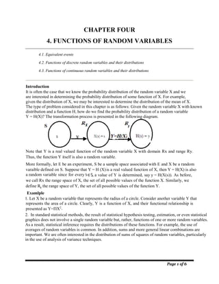
1. Page 1 of 6
CHAPTER FOUR
4. FUNCTIONS OF RANDOM VARIABLES
4.1. Equivalent events
4.2. Functions of discrete random variables and their distributions
4.3. Functions of continuous random variables and their distributions
Introduction
It is often the case that we know the probability distribution of the random variable X and we
are interested in determining the probability distribution of some function of X. For example,
given the distribution of X, we may be interested to determine the distribution of the mean of X.
The type of problem considered in this chapter is as follows: Given the random variable X with known
distribution and a function H, how do we find the probability distribution of a random variable
Y = H(X)? The transformation process is presented in the following diagram.
Note that Y is a real valued function of the random variable X with domain Rx and range Ry.
Thus, the function Y itself is also a random variable.
More formally, let E be an experiment, S be a sample space associated with E and X be a random
varaible defined on S. Suppose that Y = H (X)is a real valued function of X, then Y = H(X) is also
a random variable since for every s∈S, a value of Y is determined, say y = H(X(s)). As before,
we call Rx the range space of X, the set of all possible values of the function X. Similarly, we
define R the range space of Y, the set of all possible values of the function Y.
Examlple
1. Let X be a random variable that represents the radius of a circle. Consider another variable Y that
represents the area of a circle. Clearly, Y is a function of X, and their functional relationship is
presented as Y=X2.
2. In standard statistical methods, the result of statistical hypothesis testing, estimation, or even statistical
graphics does not involve a single random variable but, rather, functions of one or more random variables.
As a result, statistical inference requires the distributions of these functions. For example, the use of
averages of random variables is common. In addition, sums and more general linear combinations are
important. We are often interested in the distribution of sums of squares of random variables, particularly
in the use of analysis of variance techniques.
Y

2. Page 2 of 6
4.1. Equivalent events
D
De
ef
fi
in
ni
it
ti
io
on
n: Let C be an event associated with the range space of Y, RY, i.e. C . Moreover, let
 be defined as B = {x ∶ H(x)C}. Then B and C are equivalent events. Meaning, each
and every element in C is a function of a corresponding element in B.
Note
 Mathematically, if for all H(x)  C, we can find event B such that B = {x  Rx: H(x)  C}
then BC.
 When we speak of equivalent events (in the above sense), these events are associated
with different sample spaces.
1. Suppose that ( ) = . Then the events ={ >2 } ={ >4 } are equivalent.
Thus, for if Y =  X , then {X > 2}occurs if and only if {Y > 4}occurs.
Definition: Suppose X is a random variable defined on the sample space S and Rx be its range
space. Let Y=H(X) be a random variable with range space Ry. Then for any event  R , P(C) is
defined as: P(C) = P{x  R : H(x)  C}
In words :The probability of an event associated with the range space of Y is defined as the
probability of the equivalent event (in terms of X).
In other words, we can evaluate probabilities involving events associated with the function of the
random variable X if the p.d.f of X is known and if it is possible to determine the equivalent
event.Note that if B and C are equivalent events, then P (B) = P (C).
E
Ex
xa
am
mp
pl
le
e1
1:
: L
Le
et
t X
X r
re
ep
pr
re
es
se
en
nt
t t
th
he
e r
ra
ad
di
ii
i o
of
f c
ci
ir
rc
cl
le
es
s.
. S
Su
up
pp
po
os
se
e t
th
ha
at
t H
H(
(x
x)
)=
=2
2
x
x.
.
B
B1
1=
={
{x
x>
>2
2}
} i
is
s e
eq
qu
ui
iv
va
al
le
en
nt
t t
to
o C
C1
1=
={
{y
y>
>4
4
}
}
B
B2
2=
={
{x
x
5
5}
} i
is
s e
eq
qu
ui
iv
va
al
le
en
nt
t t
to
o C
C2
2=
={
{y
y
1
10
0
}
}
H
He
en
nc
ce
e,
, P
P(
(B
B1
1)
)=
=P
P(
(C
C1
1)
) a
an
nd
d P
P(
(B
B2
2)
)=
=P
P(
(C
C2
2)
)
E
Ex
xa
am
mp
pl
le
e 2
2:
: L
Le
et
t X
X b
be
e a
a c
co
on
nt
ti
in
nu
uo
ou
us
s r
ra
an
nd
do
om
m v
va
ar
ri
ia
ab
bl
le
e w
wi
it
th
h p.d.f
.


 

therwise
0
0
x
if
e
)
(
-x
O
x
f
S
Su
up
pp
po
os
se
e t
th
ha
at
t a
a r
ra
an
nd
do
om
m v
va
ar
ri
ia
ab
bl
le
e Y
Y i
is
s d
de
ef
fi
in
ne
ed
d b
by
y
2
1


X
Y .
. I
If
f =
= {Y Y
:
: 
7
7}
},
, f
fi
in
nd
d P
P(
(C
C)
).
.
2. Consider an experiment of tossing a coin twice. Let X be a random variable indicating a count for
heads. Let B= {1} be an event with respect to Rx. Then find an event A such that A B.
Example

3. Page 3 of 6
S
So
ol
lu
ut
ti
io
on
n:
:
I
It
t c
ca
an
n b
be
e s
se
ee
en
n t
th
ha
at
t R
RX
X=
= {
{ X: X>
> 0
0}
} a
an
nd
d R
RY
Y=
= {
{Y: Y >
> 1
1/
/2
2}
},
, w
wh
hi
ic
ch
h i
im
mp
pl
li
ie
es
s t
th
ha
at
t C
C
R
RY
Y.
.
15
X
7
2
1
X
7 





Y
T
Th
hu
us
s,
, d
de
ef
fi
in
ne
e B
B a
as
s B
B=
={
{X
X:
: X
X 
 1
15
5}
} s
so
o t
th
ha
at
t B
B a
an
nd
d C
C a
ar
re
e e
eq
qu
ui
iv
va
al
le
en
nt
t.
.
H
He
en
nc
ce
e,
, 15
15
1
P(B)
P(C)
e
dx
e x


 


E
Ex
xe
er
rc
ci
is
se
e:
: S
Su
up
pp
po
os
se
e t
th
ha
at
t t
th
he
e l
le
en
ng
gt
th
h o
of
f t
ti
im
me
e i
it
t t
ta
ak
ke
es
s Aaron to drive work e
ev
ve
er
ry
yd
da
ay
y i
is
s a
a r
ra
an
nd
do
om
m
v
va
ar
ri
ia
ab
bl
le
e X
X (
(m
me
ea
as
su
ur
re
ed
d i
in
n h
ho
ou
ur
rs
s)
) w
wi
it
th
h d
di
is
st
tr
ri
ib
bu
ut
ti
io
on
n f
fu
un
nc
ct
ti
io
on
n,
,








therwise
0
4
3
x
4
1
if
)
4
1
-
8(x
)
(
O
x
f
I
If
f w
we
e d
de
ef
fi
in
ne
e a
a r
ra
an
nd
do
om
m v
va
ar
ri
ia
ab
bl
le
e Y
Y a
as
s Y
Y=
=6
60
0X
X,
, t
th
he
en
n f
fi
in
nd
d P
P(
(Y
Y<
<4
45
5)
).
.
R
Re
em
ma
ar
rk
k:
: T
Th
he
e o
ot
th
he
er
r p
pr
ro
oc
ce
ed
du
ur
re
e f
fo
or
r f
fi
in
nd
di
in
ng
g p
pr
ro
ob
ba
ab
bi
il
li
it
ti
ie
es
s a
as
ss
so
oc
ci
ia
at
te
ed
d w
wi
it
th
h Y
Y i
is
s t
to
o f
fi
in
nd
d p.
.d
d.
.f
f o
of
f Y
Y
f
fr
ro
om
m t
th
he
e k
kn
no
ow
wn
n p.
.d
d.
.f
f o
of
f X
X.
.
4.2. Functions of Discrete Random Variables and their Distributions
C
Ca
as
se
e I
I:
: X
X i
is
s a
a d
di
is
sc
cr
re
et
te
e r
ra
an
nd
do
om
m v
va
ar
ri
ia
ab
bl
le
e:
:
I
If
f X
X i
is
s d
di
is
sc
cr
re
et
te
e r
ra
an
nd
do
om
m v
va
ar
ri
ia
ab
bl
le
e a
an
nd
d Y
Y=
=H
H(
(X
X)
),
, t
th
he
en
n i
it
t f
fo
ol
ll
lo
ow
ws
s i
im
mm
me
ed
di
ia
at
te
el
ly
y t
th
ha
at
t Y
Y i
is
s a
al
ls
so
o a
a
d
di
is
sc
cr
re
et
te
e r
ra
an
nd
do
om
m v
va
ar
ri
ia
ab
bl
le
e.
. T
Th
ha
at
t i
is
s, i
if
f t
th
he
e p
po
os
ss
si
ib
bl
le
e v
va
al
lu
ue
es
s o
of
f X
X a
ar
re
e x
x1
1,
,x
x2
2,
,…
…,
,x
xn
n t
th
he
en
n t
th
he
e p
po
os
ss
si
ib
bl
le
e
v
va
al
lu
ue
es
s o
of
f Y
Y a
ar
re
e H
H(
(x
x1
1)
),
,H
H(
(x
x2
2)
),
,…
…,
,H
H(
(x
xn
n)
).
.
D
De
ef
fi
in
ni
it
ti
io
on
n:
: If x , x , … , x , …. are the possible values of X, P(x ) = P(X = x ), and H is a
function such that to each value y there corresponds exactly one value x, then the probability
distribution of Y is obtained as follows:
Possible values of Y: y = H(x ), i = 1,2, … , n, …
Probabilities of Y: q(y ) = P(Y = y ) = P(x )
Example 1: Let X assumes three values: -1, 0, and 1 with probabilities 1/3, 1/2, and 1/6 respectively.
Then find the probability distributions for:
i) Y = 3X + 1
ii) Y = X + 5
Suppose that the event C is defined as C = {Y > 5}. Determine the event B such that
B= {x  Rx: H(x)  C} where Y= H(X) = 2X +1.
3

4. Page 4 of 6
Note
It may happen that several values of X lead to the same value of Y. In other words, the relation
between X and Y may not necessarily be One-to-One, as the following examples illustrate.
2. Consider the second example given above, and suppose that Y = X + 2. Then the possible values
Definition
1. Suppose that X is a discrete random variable with probability function P(X=x). Then the probability
distribution of Y = H(X) is given by P(Y=y) = P(H(X) = y) = {P(X = xi)} where H(xi) = y
2. Suppose that X is a discrete random variable with probability funtion f(x). Let Y = H(X) define a
one-to-one transformation between the values of X and Y so that the equation y = H(x) can be uniquely
solved for x in terms of y, say x = w(y). Then the probability distribution of Y is g(y) = f[w(y)].
E
Ex
xa
am
mp
pl
le
e 1
1:
: S
Su
up
pp
po
os
se
e t
th
he
e p
pr
ro
ob
ba
ab
bi
il
li
it
ty
y f
fu
un
nc
ct
ti
io
on
n o
of
f a
a d
di
is
sc
cr
re
et
te
e r
ra
an
nd
do
om
m v
va
ar
ri
ia
ab
bl
le
e X
X i
is
s
-
-1
1 0
0 1
1 2
2
(
( =
= )
) 7
7
30
30
8
8
30
30
4
4
30
30
11
11
30
30
F
Fi
in
nd
d t
th
he
e p
pr
ro
ob
ba
ab
bi
il
li
it
ty
y f
fu
un
nc
ct
ti
io
on
n o
of
f Y
Y i
if
f
a
a)
) Y
Y=
=X
X2
2
b
b)
)Y
Y=
=2
2X
X+
+5
5
Example 2: Let X be a discrete random variable having the possible values 1, 2, 3, . . . , n, . .. and
suppose that P(X = x) = . Find the probability distribution of Y if
=
1
−1
Case II: If X is a continuous random variable.
X may assume all real values while Y is defined to be +1 if > 0 and -1 if < 0. In order to
obtain the probability distribution of Y, simply determine the equivalent event (in the range
2. Suppose that X has the following probability distribution:
x: -2 -1 0 1 2 3 4
P(X=x): 0.1 0.2 0.1 0.1 0.1 0.2 0.2
Find the probability distribution of Y = 2X - 2
Example
1. Recall the first example where X assumes three values: -1, 0, and 1. If Y = X, then find the possible
values and their corresponding probabilities for Y.
2
2
of Y are 2, 3, 6, 11 and 18 with probabilities 0.1, 0.3, 0.2, 0.2 and 0.2 respectively. For example,
Y = 3 corresponds to not only one possible value in the range space of X but it refers to two possible
values, namely x = -1 and x = 1. Accordingly P(Y=3) = P(X=-1) + P(X=1) = 0.2 + 0.1

5. Page 5 of 6
space Rx) corresponding to the different values of Y. In the above case, ( = 1) = ( > 0)
and ( = −1) = ( ≤ 0).
In general case, if { = } is equivalent to an event, say A, in the range space of X, then
g( ) = ( = ) = ( )
4.3. Functions of Continuous Random Variables and their Distributions
In this section, our interest is to determine the Probability Density Function of a function of
a continuous random variable. Let X be a continuous random variable and Y be another random
variable which is a function of X. That is Y=H(X). Moreover, assume that the random variable Y
is a continuous random variable. To find or determine the p.d.f of Y=H(X), we follow the
steps below.
a) Obtain the Cumulative Distribution Function (cdf) of Y, denoted by G(y), where
( ) = (  )in terms of the cdf or p.d.f of X by finding an event A in Rx which is
equivalent to the event Yy.
b) Differentiate G(y) with respect to y in order to obtain g(y),which is going to be the p.d.f
of Y.
c) Determine those values of y in the range space of Y for which g(y)>0.
E
Ex
xa
am
mp
pl
le
e 1
1:
: S
Su
up
pp
po
os
se
e t
th
ha
at
t X
X h
ha
as
s p.d.f
. . g
gi
iv
ve
en
n b
by
y:
:








therwise
0
2
x
0
if
2
x
)
(
O
x
f
L
Le
et
t H
H(
(X
X)
)=
=2
2X
X+
+4
4.
. F
Fi
in
nd
d the p.d.f o
of
f Y
Y=
=H
H(
(X
X)
)
E
Ex
xe
er
rc
ci
is
se
e:
: L
Le
et
t a
a r
ra
an
nd
do
om
m v
va
ar
ri
ia
ab
bl
le
e X
X h
ha
as
s a
a d
de
en
ns
si
it
ty
y f
fu
un
nc
ct
ti
io
on
n


 


therwise
0
1
x
0
if
1
)
(
O
x
f .
. L
Le
et
t
H
H(
(X
X)
)=
=e
ex
x
.
. T
Th
he
en
n f
fi
in
nd
d t
th
he
e p.d.f o
of
f Y
Y=
=H
H(
(X
X)
).
.
Example: suppose that X has the pdf
f(x) =
2x, 0 < < 1
0 otherwise
Solution:
If Y = 3X + 1, then find the pdf of Y

6. Page 6 of 6
The other method of obtaining ( ).
( ) = ( ≤ ) = ≤
− 1
3
=
− 1
3
,
Where F is the cdf of X; that is
( ) = ( ≤ ).
In order to calculate the derivative of G, ( ), we use the chain rule for differentiation as
follows:
( ) =
( ) = ( ) ; ℎ =
− 1
3
Hence
( ) = ( ) ∗
1
3
= ( ) ∗
1
3
= 2 ∗
− 1
3
∗
1
3
=
2
9
( − 1)
Theorem: Let X be a continuous random variable with pdf , where ( ) > 0 for < <
. suppose that = ( ) is a strictly monotone (increasing or decreasing) function of . Assume
that this function is differentiable ( and hence continuous) for all . Then the random variable Y
defined as = ( )has a pdf g given by,
( ) = (H (y)) ∗ H (y) ℎ H (y) = x
Example
Theorem: Let X be a continuous random variable with pdf f and Y = . Then the random
variable Y has the pdf given by: g(y) =
1
2 [f( ]
y ) + f(
2. Suppose that the pdf of a random variable X is given by: f(x) = 1 0 < x < 1
0 otherwise
Find the pdf of Y = ln(X)
- )
-1
Find the pdf of Y = e
Let the pdf of X is given as f(x) = 1/2 if -1 < x < 1, and 0 else where. If Y = 4 - X, then find
the pdf of Y.
2
1. Let X be a random variable with pdf: f(x) = 
otherwise
x 0 < x < 1
-x
{
Example