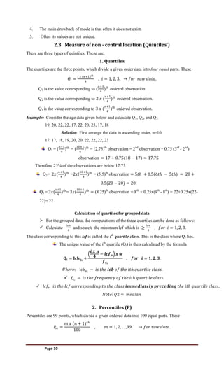
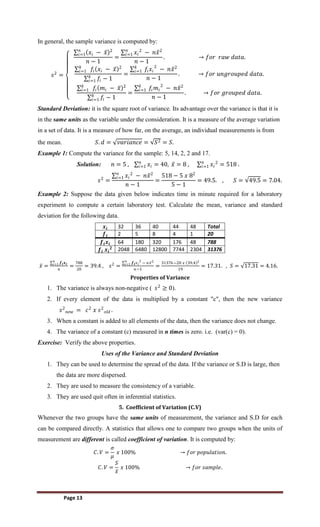
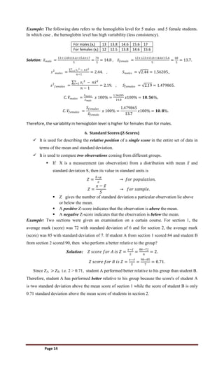
The document discusses measures of central tendency and summarization of data. It defines measures of central tendency as single values that describe the overall level of a data set and represent the center of the distribution. The most common measures are the mean, median, and mode. It provides formulas for calculating the arithmetic mean for samples and populations. It also introduces summation notation as a shorthand for writing sums and discusses properties of summation. Examples are provided to demonstrate calculating the mean for raw data, ungrouped data, and grouped data. The document also discusses calculating a combined mean for multiple data sets.
To arrange the data in such a way that it should create interest in the readerโs mind at the first sight.
To present the information in a compact and concise form without losing important details.
In the previous lesson we discussed a measure of location known as the measure of central tendency. There are other measures of location which are useful in describing the distribution of the data set. These measures of location include the maximum, minimum, percentiles, deciles and quartiles. How to compute and interpret these measures are also discussed in this lesson.
๏บPlease Subscribe to this Channel for more solutions and lectures
http://www.youtube.com/onlineteaching
Chapter 6: Normal Probability Distribution
6.3: Sampling Distributions and Estimators
Measure of central tendency provides a very convenient way of describing a set of scores with a single number that describes the PERFORMANCE of the group.
It is also defined as a single value that is used to describe the โcenterโ of the data.
๏บPlease Subscribe to this Channel for more solutions and lectures
http://www.youtube.com/onlineteaching
Elementary Statistics Practice Test 1
Module 1: Chapters 1-3
Chapter 1: Introduction to Statistics.
Chapter 2: Exploring Data with Tables and Graphs.
Chapter 3: Describing, Exploring, and Comparing Data.
An ahp (analytic hierarchy process)fce (fuzzy comprehensive evaluation) based...ijcsa
ย
In this paper the AHP (Analytic Hierarchy Process) and the FCE (Fuzzy Comprehensive Evaluation) are
applied to find the best coaches from different sports and to rank these great coaches.
First, we screen coachesโ information using three screening criterions. We rank the screened coaches
preliminarily by means of analytic hierarchy process (AHP). Second, we rank them by fuzzy comprehensive
evaluation method(FCE), and we determined the top5 coaches on basketball, football and hockey. Third,
we use the Topsis method to test the accuracy and reasonableness of the model, modify the model and then
reorder the original results to inspect the consistency of the results of the two models. Finally, we take
some other factors into account to optimize our model, which includes on the influence of time line horizon
and genders.
Central tendency of data is defined as the tendency of data to concentrate around some central value. here all the measures of central tendency have been explained such as mean, arithmetic mean, geometric mean, harmonic mean, mode, and median with examples.
Measures of Central tendency-bio-statistics
Biostatistics and research methodology
Mean
Median
Mode
Mean- Arithmetic mean
weighted mean
harmonic mean
geometric mean
individual series
discrete series
continuous series
Relation between mean, median and mode
Statistical average
mathematical average
positional average
Merits and demerits of mean, median and mode
statistics
Bachelor of Pharmacy
8th Semester
Biostatistics
Comparative analysis of x^3+y^3=z^3 and x^2+y^2=z^2 in the Interconnected Sets Vladimir Godovalov
ย
This paper introduces an innovative technique of study z^3-x^3=y^3 on the subject of its insolvability in integers. Technique starts from building the interconnected, third degree sets: A3={a_nโa_n=n^3,nโN}, B3={b_nโb_n=a_(n+1)-a_n }, C3={c_nโc_n=b_(n+1)-b_n } and P3={6} wherefrom we get a_n and b_n expressed as figurate polynomials of third degree, a new finding in mathematics. This approach and the results allow us to investigate equation z^3-x^3=y in these interconnected sets A3 and B3, where z^3โงx^3โA3, yโB3. Further, in conjunction with the new Method of Ratio Comparison of Summands and Pascalโs rule, we finally prove inability of y=y^3. After we test the technique, applying the same approach to z^2-x^2=y where we get family of primitive z^2-x^2=y^2 as well as introduce conception of the basic primitiveness of z^'2-x^'2=y^2 for z^'-x^'=1 and the dependant primitiveness of z^'2-x^'2=y^2 for co-prime x,y,z and z^'-x^'>1.
Many Decision Problems in business and social systems can be modeled using mathematical optimization, which seeks to maximize or minimize some objective which is a function of the decisions.
Stochastic Optimization Problems are mathematical programs where some of the data incorporated into the objective or constraints are Uncertain.
whereas, Deterministic Optimization Problems are formulated with known parameters.
The owner is required by law to:
o post the fire safety plan on the inside of every apartment front door.
o post the fire safety plan in a conspicuous space in the common area.
o distribute a copy to each dwelling unit in the building.
o provide a copy to new tenants at the time of the lease.
o re-distribute the fire safety plan annually during fire prevention week
The figure shows the section of a gravity dam built with concrete. Examine the stability of this section at the base. The earthquake forces may be taken as equivalent to 0.1g for horizontal forces and 0.05g for vertical forces. The uplift may be taken as equal to the hydrostatic pressure at the either ends and is considered to act over 60% of the area of the section. 1 in 10 6m A tail water depth of 6m is assumed to be present when the reservoir is full and there is no tail water when the reservoir is empty. Also indicate the values of various kinds of stresses that are developed at heel and toe. Assume weight of concrete = 24 kN/mยณ; and weight of water = 10 kN/mยณ
tend to form in some materials
โข
Since
the fine materials are usually sensitive to moisture
the field Engineer must be extremely weather
conscious
โข
If
heavy rain is expected the surface of the fine material
should be rolled smooth with sufficient gradient to shed
water from the working area
great deal from general to highly specialized applications. A contractor engaged in highway construction must usually drill rock under varying conditions; therefore, equipment that is suitable for various services would be selected.
Purposes for which drilling are performed vary a great deal from performed vary a great deal from general to highly specialized general to highly specialized applications applications. It is desirable to select the It is desirable to select the equipment and methods that are equipment and methods that are best suited to the specific service:
11. A concrete dam can be assumed to be trapezoidal in section having a top width of 2 m and bottom width of 10 m. Its height is 12 m and the upstream face has a batter of 1: 10. Give an analysis of the stability of the dam for the base section for overturning and sliding in the full reservoir condition assuming no free-board allowance but allowing for uplift pressures. Assume uplift intensity factor ast 100%. Also determine the compressive stresses at the toe and the heel, and major principal and shear stress developed at the toe. Assume weight of concrete to be 24 kN/mยณ, unit shear strength of concrete
to be 1400 KN/mยณ, and the coefficient of friction between concrete and foundation soil to be 0.7.
12. The following data refer to the non-overflow section of a gravity dam:
R.L. of top of the dam
315 m.
R.L. of bottom of the dam
260 m
Full reservoir level
= 312 m
Top width of the dam
= 12 m.
Unstream face is vertical. Downstream face is vertical upto R.L. 304 m; and thereafter, the
Opendatabay - Open Data Marketplace.pptxOpendatabay
ย
Opendatabay.com unlocks the power of data for everyone. Open Data Marketplace fosters a collaborative hub for data enthusiasts to explore, share, and contribute to a vast collection of datasets.
First ever open hub for data enthusiasts to collaborate and innovate. A platform to explore, share, and contribute to a vast collection of datasets. Through robust quality control and innovative technologies like blockchain verification, opendatabay ensures the authenticity and reliability of datasets, empowering users to make data-driven decisions with confidence. Leverage cutting-edge AI technologies to enhance the data exploration, analysis, and discovery experience.
From intelligent search and recommendations to automated data productisation and quotation, Opendatabay AI-driven features streamline the data workflow. Finding the data you need shouldn't be a complex. Opendatabay simplifies the data acquisition process with an intuitive interface and robust search tools. Effortlessly explore, discover, and access the data you need, allowing you to focus on extracting valuable insights. Opendatabay breaks new ground with a dedicated, AI-generated, synthetic datasets.
Leverage these privacy-preserving datasets for training and testing AI models without compromising sensitive information. Opendatabay prioritizes transparency by providing detailed metadata, provenance information, and usage guidelines for each dataset, ensuring users have a comprehensive understanding of the data they're working with. By leveraging a powerful combination of distributed ledger technology and rigorous third-party audits Opendatabay ensures the authenticity and reliability of every dataset. Security is at the core of Opendatabay. Marketplace implements stringent security measures, including encryption, access controls, and regular vulnerability assessments, to safeguard your data and protect your privacy.
Show drafts
volume_up
Empowering the Data Analytics Ecosystem: A Laser Focus on Value
The data analytics ecosystem thrives when every component functions at its peak, unlocking the true potential of data. Here's a laser focus on key areas for an empowered ecosystem:
1. Democratize Access, Not Data:
Granular Access Controls: Provide users with self-service tools tailored to their specific needs, preventing data overload and misuse.
Data Catalogs: Implement robust data catalogs for easy discovery and understanding of available data sources.
2. Foster Collaboration with Clear Roles:
Data Mesh Architecture: Break down data silos by creating a distributed data ownership model with clear ownership and responsibilities.
Collaborative Workspaces: Utilize interactive platforms where data scientists, analysts, and domain experts can work seamlessly together.
3. Leverage Advanced Analytics Strategically:
AI-powered Automation: Automate repetitive tasks like data cleaning and feature engineering, freeing up data talent for higher-level analysis.
Right-Tool Selection: Strategically choose the most effective advanced analytics techniques (e.g., AI, ML) based on specific business problems.
4. Prioritize Data Quality with Automation:
Automated Data Validation: Implement automated data quality checks to identify and rectify errors at the source, minimizing downstream issues.
Data Lineage Tracking: Track the flow of data throughout the ecosystem, ensuring transparency and facilitating root cause analysis for errors.
5. Cultivate a Data-Driven Mindset:
Metrics-Driven Performance Management: Align KPIs and performance metrics with data-driven insights to ensure actionable decision making.
Data Storytelling Workshops: Equip stakeholders with the skills to translate complex data findings into compelling narratives that drive action.
Benefits of a Precise Ecosystem:
Sharpened Focus: Precise access and clear roles ensure everyone works with the most relevant data, maximizing efficiency.
Actionable Insights: Strategic analytics and automated quality checks lead to more reliable and actionable data insights.
Continuous Improvement: Data-driven performance management fosters a culture of learning and continuous improvement.
Sustainable Growth: Empowered by data, organizations can make informed decisions to drive sustainable growth and innovation.
By focusing on these precise actions, organizations can create an empowered data analytics ecosystem that delivers real value by driving data-driven decisions and maximizing the return on their data investment.
Adjusting primitives for graph : SHORT REPORT / NOTESSubhajit Sahu
ย
Graph algorithms, like PageRank Compressed Sparse Row (CSR) is an adjacency-list based graph representation that is
Multiply with different modes (map)
1. Performance of sequential execution based vs OpenMP based vector multiply.
2. Comparing various launch configs for CUDA based vector multiply.
Sum with different storage types (reduce)
1. Performance of vector element sum using float vs bfloat16 as the storage type.
Sum with different modes (reduce)
1. Performance of sequential execution based vs OpenMP based vector element sum.
2. Performance of memcpy vs in-place based CUDA based vector element sum.
3. Comparing various launch configs for CUDA based vector element sum (memcpy).
4. Comparing various launch configs for CUDA based vector element sum (in-place).
Sum with in-place strategies of CUDA mode (reduce)
1. Comparing various launch configs for CUDA based vector element sum (in-place).
Techniques to optimize the pagerank algorithm usually fall in two categories. One is to try reducing the work per iteration, and the other is to try reducing the number of iterations. These goals are often at odds with one another. Skipping computation on vertices which have already converged has the potential to save iteration time. Skipping in-identical vertices, with the same in-links, helps reduce duplicate computations and thus could help reduce iteration time. Road networks often have chains which can be short-circuited before pagerank computation to improve performance. Final ranks of chain nodes can be easily calculated. This could reduce both the iteration time, and the number of iterations. If a graph has no dangling nodes, pagerank of each strongly connected component can be computed in topological order. This could help reduce the iteration time, no. of iterations, and also enable multi-iteration concurrency in pagerank computation. The combination of all of the above methods is the STICD algorithm. [sticd] For dynamic graphs, unchanged components whose ranks are unaffected can be skipped altogether.
StarCompliance is a leading firm specializing in the recovery of stolen cryptocurrency. Our comprehensive services are designed to assist individuals and organizations in navigating the complex process of fraud reporting, investigation, and fund recovery. We combine cutting-edge technology with expert legal support to provide a robust solution for victims of crypto theft.
Our Services Include:
Reporting to Tracking Authorities:
We immediately notify all relevant centralized exchanges (CEX), decentralized exchanges (DEX), and wallet providers about the stolen cryptocurrency. This ensures that the stolen assets are flagged as scam transactions, making it impossible for the thief to use them.
Assistance with Filing Police Reports:
We guide you through the process of filing a valid police report. Our support team provides detailed instructions on which police department to contact and helps you complete the necessary paperwork within the critical 72-hour window.
Launching the Refund Process:
Our team of experienced lawyers can initiate lawsuits on your behalf and represent you in various jurisdictions around the world. They work diligently to recover your stolen funds and ensure that justice is served.
At StarCompliance, we understand the urgency and stress involved in dealing with cryptocurrency theft. Our dedicated team works quickly and efficiently to provide you with the support and expertise needed to recover your assets. Trust us to be your partner in navigating the complexities of the crypto world and safeguarding your investments.
As Europe's leading economic powerhouse and the fourth-largest hashtag#economy globally, Germany stands at the forefront of innovation and industrial might. Renowned for its precision engineering and high-tech sectors, Germany's economic structure is heavily supported by a robust service industry, accounting for approximately 68% of its GDP. This economic clout and strategic geopolitical stance position Germany as a focal point in the global cyber threat landscape.
In the face of escalating global tensions, particularly those emanating from geopolitical disputes with nations like hashtag#Russia and hashtag#China, hashtag#Germany has witnessed a significant uptick in targeted cyber operations. Our analysis indicates a marked increase in hashtag#cyberattack sophistication aimed at critical infrastructure and key industrial sectors. These attacks range from ransomware campaigns to hashtag#AdvancedPersistentThreats (hashtag#APTs), threatening national security and business integrity.
๐ Key findings include:
๐ Increased frequency and complexity of cyber threats.
๐ Escalation of state-sponsored and criminally motivated cyber operations.
๐ Active dark web exchanges of malicious tools and tactics.
Our comprehensive report delves into these challenges, using a blend of open-source and proprietary data collection techniques. By monitoring activity on critical networks and analyzing attack patterns, our team provides a detailed overview of the threats facing German entities.
This report aims to equip stakeholders across public and private sectors with the knowledge to enhance their defensive strategies, reduce exposure to cyber risks, and reinforce Germany's resilience against cyber threats.
Levelwise PageRank with Loop-Based Dead End Handling Strategy : SHORT REPORT ...Subhajit Sahu
ย
Abstract โ Levelwise PageRank is an alternative method of PageRank computation which decomposes the input graph into a directed acyclic block-graph of strongly connected components, and processes them in topological order, one level at a time. This enables calculation for ranks in a distributed fashion without per-iteration communication, unlike the standard method where all vertices are processed in each iteration. It however comes with a precondition of the absence of dead ends in the input graph. Here, the native non-distributed performance of Levelwise PageRank was compared against Monolithic PageRank on a CPU as well as a GPU. To ensure a fair comparison, Monolithic PageRank was also performed on a graph where vertices were split by components. Results indicate that Levelwise PageRank is about as fast as Monolithic PageRank on the CPU, but quite a bit slower on the GPU. Slowdown on the GPU is likely caused by a large submission of small workloads, and expected to be non-issue when the computation is performed on massive graphs.
Ch03-Managing the Object-Oriented Information Systems Project a.pdf
ย
Ch2
1. Page 1
CHAPTER - 2
2. Summarization of Data
2.1 Measures of Central Tendency
The most important objective of a statistical analysis is to determine a single value for the entire
mass of data, which describes the overall level of the group of observations and can be called a
representative of the whole set of data. It tells us where the center of the distribution of data is
located. The most commonly used measures of central tendencies are :
๏ผ The Mean (Arithmetic mean, Weighted mean, Geometric mean and Harmonic means)
๏ผ The Mode
๏ผ The Median
The Summation Notation:
๏ง Let ๐1, ๐2, โฆ , ๐๐ be the number of measurements where ๐ is the total number of
observation and ๐๐, is the ith
observation.
๏ง Very often in statistics an algebraic expression of the form ๐1 + ๐2 + โฏ + ๐๐ is used in
a formula to compute a statistic. It is tedious to write an expression like this very often,
so mathematicians have developed a shorthand notation to represent a sum of scores,
called the summation notation.
๏ง The symbol ๐๐
๐
๐=1 is a mathematical shorthand for ๐1 + ๐2 + โฏ + ๐๐.
๐๐๐๐๐๐๐๐๐, ๐ฟ๐
๐ต
๐=๐ = ๐ฟ๐ + ๐ฟ๐ + โฏ + ๐ฟ๐ต โ ๐๐๐ ๐ก๐๐ ๐๐๐๐ข๐๐๐ก๐๐๐๐ .
๐ฟ๐
๐
๐=๐ = ๐ฟ๐ + ๐ฟ๐ + โฏ + ๐ฟ๐ โ ๐๐๐ ๐ก๐๐ ๐ ๐๐๐๐๐๐ .
Example: Suppose the following were scores (marks) made on the first assignment for
five students in the class: 5, 7, 7, 6, ๐๐๐ 8. Write their marks using summation notation.
Solution: ๐๐
5
๐=1 = ๐1 + ๐2 + โฏ + ๐5 = 5 + 7 + 7 + 6 + 8 = 33
Properties of summation
1. ๐
๐
๐=1 = ๐๐ ๐๐๐ ๐๐๐ฆ ๐๐๐๐ ๐ก๐๐๐ก ๐.
2. ๐๐๐
๐
๐=1 = ๐ ๐๐
๐
๐=1
3. (๐๐ ยฑ ๐)
๐
๐=1 = ๐๐
๐
๐=1 ยฑ ๐๐
4. (๐๐+๐๐)
๐
๐=1 = ๐๐
๐
๐=1 + ๐๐
๐
๐=1
5. ๐๐๐๐
๐
๐=1 = ๐1๐1 + ๐2๐2 + โฏ + ๐๐๐๐
6. 1 + 2 + 3 + 4 + โฏ + ๐ =
๐(๐+1)
2
7. 12
+ 22
+32
+ โฏ + ๐2
=
๐ ๐+1 (2๐+1)
6
2.2 Types of Measure of Central Tendency
2.2.1 The Mean
2.2.1.1 Arithmetic mean
The arithmetic mean of a sample is the sum of all observations divided by the number of
observations in the sample. i.e.
๐บ๐๐๐๐๐ ๐๐๐๐ ๐๐ ๐๐๐๐๐๐๐๐๐๐ ๐๐๐๐ =
๐๐๐ ๐๐๐ ๐๐ ๐๐๐ ๐๐๐๐๐๐ ๐๐ ๐๐๐ ๐๐๐๐๐๐
๐๐๐๐๐๐ ๐๐ ๐๐๐๐๐๐ ๐๐ ๐๐๐ ๐๐๐๐๐๐
Suppose that ๐ฅ1, ๐ฅ2, โฆ , ๐ฅ๐ are n observed values in a sample of size n taken from a population
of size N. Then the arithmetic mean of the sample, denoted by ๐ฅ, is given by
2. Page 2
๐ฟ =
๐ฟ๐+๐ฟ๐+โฏ+๐ฟ๐
๐ง
=
๐ฟ๐
๐
๐=๐
๐
โ ๐๐จ๐ซ ๐ฌ๐๐ฆ๐ฉ๐ฅ๐๐ฌ.
If we take an entire population, the population mean denoted by ยต is given by
ยต =
๐ฟ๐+๐ฟ๐+โฏ+๐ฟ๐ต
๐
=
๐ฟ๐
๐ต
๐=๐
๐ต
โ ๐๐จ๐ซ ๐ฉ๐จ๐ฉ๐ฎ๐ฅ๐๐ญ๐ข๐จ๐ง๐ฌ.
In general, the sample arithmetic mean is calculated by
๐ฟ =
๐ฟ๐
๐
๐
๐=๐ โ ๐๐๐ ๐๐๐ค ๐๐ก๐๐ก๐
๐๐๐ฟ๐
๐๐
๐
๐=๐ โ ๐๐๐ ๐ข๐๐๐๐๐ข๐๐๐ ๐๐๐ก๐ ๐ค๐๐๐๐ ๐๐ = ๐.
๐ด๐๐ฟ๐
๐๐
๐
๐=๐ โ ๐๐๐ ๐๐๐๐ข๐๐๐ ๐๐๐ก๐ ๐ค๐๐๐๐ ๐๐ = ๐.
Example 1: The net weights of five perfume bottles selected at random from the production
line ๐๐๐ 85.4, 85.3, 84.9, 85.4 ๐๐๐ 85. What is the arithmetic mean weight of the sample
observation?
Solution; ๐บ๐๐ฃ๐๐ ๐ = 5 ๐ฅ1 = 85.4, ๐ฅ2 = 85.3, ๐ฅ3 = 84.9, ๐ฅ4 = 85.4 ๐๐๐ ๐ฅ5 = 85.
๐ =
๐๐
๐
๐=1
๐
=
85.4+85.3+84.9+85.4+ 85
5
=
426.6
5
= 85.32.
Example 2: Calculate the mean of the marks of 46 students given below;
Marks (๐๐) 9 10 11 12 13 14 15 16 17 18
Frequency (๐๐) 1 2 3 6 10 11 7 3 2 1
Solution: ๐๐ = ๐ = 46 is the sum of the frequencies or total number of observations.
To calculate ๐๐๐ฟ๐
๐
๐=1 consider the following table.
๐๐ 9 10 11 12 13 14 15 16 17 18 Total
๐๐ 1 2 3 6 10 11 7 3 2 1 46
๐๐๐ฟ๐ 9 20 33 72 130 154 105 48 34 18 623
So ๐ =
๐๐๐ฟ๐
๐๐
๐
๐=๐ =
623
46
= 13.54.
Example 3: The net income of a sample of large importers of Urea was organized into the
following table. What is the arithmetic mean of net income?
Net income 2-4 5-7 8-10 11-13 14-16
Number of importers 1 4 10 3 2
Solution: ๐๐ = ๐ = 20 is the sum of the frequencies or total number of observations.
To calculate ๐๐๐๐
๐
๐=1 consider the following table.
Net income (CI) 2-4 5-7 8-10 11-13 14-16 Total
Number of importers (๐๐) 1 4 10 3 2 20
Class marks (๐๐) 3 6 9 12 15
๐๐๐๐ 3 24 90 36 30 183
So ๐ =
๐๐๐๐
๐๐
๐
๐=๐ =
๐๐๐
๐๐
= ๐. ๐๐.
Example 4: From the following data, calculate the missing frequency? The mean number of
tablets to cure ever was 29.18.
Number of tablets 19 โ 21 22 โ 24 25 โ 27 28 โ 30 31 โ 33 34 โ 36 37 โ 39
Number of persons cured 6 13 19 ๐4 18 12 9
3. Page 3
Solution; ๐๐ = ๐ = 77 + ๐
4 is the sum of the frequencies or total number of observations.
To calculate ๐๐๐๐
๐
๐=1 consider the following table.
CI 19 โ 21 22 โ 24 25 โ 27 28 โ 30 31 โ 33 34 โ 36 37 โ 39 Total
๐๐ 6 13 19 ๐4 18 12 9 77+๐
4
๐๐ 20 23 26 29 32 35 38
๐๐๐๐ 120 299 494 29๐4 576 420 342 2251 + 29๐4
๐๐๐๐๐ ๐๐๐๐ ๐๐ ๐๐๐ฃ๐๐ ๐ก๐ ๐๐ 29.18 ๐ค๐ ๐๐๐ฃ๐
๐ =
๐๐๐๐
๐๐
๐
๐=1
=โซ 29.18 =
2251 + 29๐
4
77+๐
4
=โซ 29.18 77+๐
4 = 2251 + 29๐
4
=โซ 29.18๐
4 โ 29๐4 = 2251 โ 2246.86 =โซ 0.18๐
4 = 4.14 =โซ ๐
4 =
4.14
0.18
= 23.
Combined mean
If we have an arithmetic means ๐1, ๐2, โฆ , ๐๐ of n groups having the same unit of measurement
of a variable, with sizes ๐1, ๐2, โฆ , ๐๐ observations respectively, we can compute the combined
mean of the variant values of the groups taken together from the individual means by
๐ฟ๐๐๐ =
๐๐๐๐+๐๐๐๐+โฏ+๐๐๐๐
๐๐+๐๐+โฏ+๐๐
=
๐๐๐๐
๐
๐=๐
๐๐
๐
๐=๐
Example 1: Compute the combined mean for the following two sets.
๐บ๐๐ ๐จ: 1, 4, 12, 2, 8 ๐๐๐ 6 ; ๐บ๐๐ ๐ฉ: 3, 6, 2, 7 ๐๐๐ 4.
Solution: ๐1 = 6, ๐ฅ1 =
๐๐
6
๐=1
๐๐
=
33
6
= 5.5 ; ๐2 = 6, ๐ฅ2 =
๐๐
5
๐=1
๐๐
=
22
5
= 4.4.
๐๐๐๐ =
๐1๐ฅ1 + ๐2๐ฅ2
๐1 + ๐2
=
6 ๐ฅ 5.5 + 5 ๐ฅ 4.4
6 + 5
=
55
11
= 5.
Example 2: The mean weight of 150 students in a certain class is 60 kg. The mean
weight of boys in the class is 70 kg and that of girlโs is 55 kg . Find the number of boys
and girls in the class?
Solution; Let ๐1 be the number of boys and ๐2 be the number of girls in the class.
Also let ๐ฅ1 , ๐ฅ2 ๐๐๐ ๐ฅ๐๐๐ be the mean weights of boys, girls and the mean weights of all
students respectively. Then ๐ฅ1 = 70, ๐ฅ2 = 55 ๐๐๐ ๐ฅ๐๐๐ = 60. ๐ถ๐๐๐๐๐๐ฆ ๐1 + ๐2 = 150.
๐๐๐๐ =
๐1๐ฅ1+๐2๐ฅ2
๐1+๐2
=โซ 60 =
70 ๐1+55๐2
๐1+๐2
=โซ 60 =
70 ๐1+55๐2
150
=โซ 9000 = 70 ๐1 + 55๐2 โฆ . โฆ 1 ๐๐๐
150 = ๐1 + ๐2 โฆ โฆ (2)
๐๐๐๐ฃ๐๐๐ ๐๐๐ข๐๐ก๐๐๐ (1) ๐๐๐ (2) ๐ ๐๐๐ข๐๐ก๐๐๐๐๐ข๐ ๐๐ฆ, ๐ค๐ ๐๐๐ก ๐1 = 50 ๐๐๐ ๐2 = 100.
Disadvantages of the arithmetic mean
1. The mean is meaningless in the case of nominal or qualitative data.
2. In case of grouped data, if any class interval is open ended, arithmetic mean cannot be
calculated, since the class mark of this interval cannot be found.
2.2.1.2 Weighted mean
In the computation of arithmetic mean, we had given an equal importance to each observation.
Sometimes the individual values in the data may not have an equally importance. When this is
the case, we assigned to each weight which is proportional to its relative importance.
๏ The weighted mean of a set of values ๐ฅ1, ๐ฅ2, โฆ , ๐ฅ๐ with corresponding weights
๐ค1, ๐ค2, โฆ , ๐ค๐ denoted by ๐ฅ๐ค is computed by:
4. Page 4
๐ฟ๐ =
๐๐๐๐ + ๐๐๐๐ + โฏ + ๐๐๐๐
๐๐ + ๐๐ + โฏ + ๐๐
=
๐๐๐๐
๐
๐=๐
๐๐
๐
๐=๐
The calculation of cumulative grade point average (CGPA) in Colleges and Universities is a
good example of weighted mean.
Example: If a student scores "A" in a 3 EtCTS course, "B" in a 6 EtCTS course, "B" in
another 5 EtCTS course and "D" in a 2 EtCTS course. Compute his /her GPA for the semester.
Solution: Here the numerical values of the letter grades are the values (i.e. ๐ด = 4, ๐ต =
3, ๐ถ = 2 ๐๐๐ ๐ท = 1) and the corresponding EtCTS of the course are their respective
weights. i.e.
Grade values (๐๐) 4 3 3 1
Weight (๐๐) 3 6 5 2
๐ฎ๐ท๐จ = ๐ฟ๐ =
๐๐๐๐+๐๐๐๐+โฏ+๐๐๐๐
๐๐+๐๐+โฏ+๐๐
=
๐๐๐๐
๐
๐=๐
๐๐
๐
๐=๐
=
4x3+3x6+3x5+1x2
3+6+5+2
=
12+18+15+2
16
=
47
16
= 2.9375.
2.2.1.3 Geometric mean
In algebra geometric mean is calculated in the case of geometric progression, but in statistics we
need not bother about the progression, here it is particular type of data for which the geometric
mean is of great importance because it gives a good mean value. If the observed values are
measured as ratios, proportions or percentages, then the geometric mean gives a better measure
of central tendency than any other means.
๏ The Geometrical mean of a set of values ๐ฅ1, ๐ฅ2, โฆ , ๐ฅ๐ of n positive values is defined as the
nth
root of their product . That is,
๐บ. ๐ = ๐ฅ1 โ ๐ฅ2 โ โฆ โ ๐ฅ๐
๐
Example: The G.M of 4, 8 and 6 is
๐บ. ๐ = 4 ๐ฅ 8 ๐ฅ 6
3
= 192
3
= 5.77.
In general, the sample geometric mean is calculated by
๐ฎ. ๐ =
๐ฅ1 โ ๐ฅ2 โ โฆ โ ๐ฅ๐
๐
โ ๐๐๐ ๐๐๐ค ๐๐ก๐๐ก๐
๐ฅ1
๐1 โ ๐ฅ2
๐2 โ, โฆ ,โ ๐ฅ๐
๐๐
๐
โ ๐๐๐ ๐ข๐๐๐๐๐ข๐๐๐ ๐๐๐ก๐ ๐ค๐๐๐๐ ๐ = ๐๐ .
๐1
๐1 โ ๐2
๐2 โ. , โฆ ,โ ๐๐
๐๐
๐
โ ๐๐๐ ๐๐๐๐ข๐๐๐ ๐๐๐ก๐ ๐ค๐๐๐๐ ๐ = ๐๐ .
Example1: The man gets three annual raises in his salary. At the end of first year, he
gets an increase of 4%, at the end of the second year, he gets an increase of 6% and at the
end of the third year, he gets an increase of 9% of his salary. What is the average
percentage increase in the three periods?
Solution: ๐บ. ๐ = 1.04 โ 1.06 โ 1.09
3
= 1.0631 => 1.0631 โ 1 = 0.0631.
๐๐๐๐๐๐๐๐๐, ๐ก๐๐ ๐๐ฃ๐๐๐๐๐ ๐๐๐๐๐๐๐ก๐๐๐ ๐๐๐๐๐๐๐ ๐ ๐๐ 6.31%.
Example 2: Compute the Geometric mean of the following data.
Values 2 4 6 8 10
Frequency 1 2 2 2 1
5. Page 5
๐บ๐๐๐๐๐๐๐: ๐. ๐ = 21 โ 42 โ 62 โ 82 โ 101
8
= 2 โ 16 โ 36 โ 64 โ 100
8
= 737280
8
= 5.41.
Example 3: Suppose that the profits earned by a certain construction company in four projects
were 3%, 2%, 4% & 6% respectively. What is the Geometric mean profit?
๐บ๐๐๐๐๐๐๐: ๐. ๐ = 3 โ 2 โ 4 โ 6
4
= 144
4
= 3.46.
๐๐๐๐๐๐๐๐๐; ๐ก๐๐ ๐๐๐๐๐๐ก๐๐๐ ๐๐๐๐ ๐๐๐๐๐๐ก ๐๐ 3.46 ๐๐๐๐๐๐๐ก.
2.2.1.4 Harmonic mean
Another important mean is the harmonic mean, which is suitable measure of central tendency
when the data pertains to speed, rates and price.
๏ Let ๐ฅ1, ๐ฅ2, โฆ , ๐ฅ๐ be n variant values in a set of observations, then simple harmonic
mean is given by: ๐บ. ๐ฏ. ๐ด =
๐ง
๐
๐ฑ๐
+
๐
๐ฑ๐
+โฏ+
๐
๐ฑ๐ง
=
๐ง
๐
๐ฑ๐ข
๐ง
๐ข=๐
๏ผ Note: SHM is used for equal distances, equal costs and equal rates.
Example 1: A motorist travels for three days at a rate (speed) of 480 km/day. On the first day he
travels 10 hours at a rate of 48 km/h, on the second day 12 hours at a rate of 40 km/h, on the
third day 15 hours at a rate of 32 km/h. What is the average speed?
Solution: Since the distance covered by the motorist is equal (๐. ๐. ๐ 1 = 480, ๐ 2 = 480, ๐ 3 =
480), so we use SHM.
๐. ๐ป. ๐ =
3
1/48+1/40+1/32
= 38.92 so the required average speed = 38.92 ๐๐/๐.
We can check this, by using the known formula for average speed in elementary physics.
Check; ๐ด๐ฃ๐๐๐๐๐ ๐ ๐๐๐๐ ๐
๐๐ฃ =
total distance covered
total time taken
=
๐๐
๐ก๐
=
480km +480km +480km
10hr+12hr+15hr
=
1440km
37hr
= 38.42 ๐๐/ h.
Example 2: A business man spent 20 Birr for milk at 40 cents per liter in Mizan-Aman town and
another 20 Birr at 60 cents per liter in Tepi town. What is the average price of milk at two towns.
Solution: Since the price on the two towns are equal (20 Birr), so we use SHM.
๐ด๐ฃ๐๐๐๐๐ ๐๐๐๐๐ (๐๐๐ฃ ) = ๐. ๐ป. ๐ =
2
1
40
+
1
60
= 48 ๐๐๐๐ก๐ /๐๐๐ก๐๐.
Weighted harmonic mean (WHM)
๏ผ WHM is used for different distance, different cost and different rate.
๐. ๐ป. ๐ =
๐ค๐
wi
xi
Example 1: A driver travel for 3 days. On the 1st
day he drives for 10h at a speed of 48 km/h, on
the 2nd
day for 12h at 45 km/h and on the 3rd day for 15h at 40 km/h. What is the average speed?
Solution: since the distance covered by the driver is not equal, so we use WHM by taking
the distance as weights (wi).
๐ฃ๐๐ฃ = ๐ค. ๐. ๐ =
๐ค๐
wi
xi
=
(480 + 540 + 600)๐๐
480
40 +
540
45
+
600
40 ๐๐
= 43.32 ๐๐/๐๐.
Example 2: A business man spent 20 Birr for milk at rate of 40 cents per liter in Mizan-Aman
town and 25 Birr at a price of 50 cents per liter in Tepi town. What is the average price ?
6. Page 6
Solution: Since the price on the two towns are different , so we use WHM by taking the cost as
weights (wi).
๐๐๐ฃ = ๐ค. ๐. ๐ =
๐ค๐
wi
xi
=
20 + 25 ๐๐๐๐
20
40
+
25
50
๐๐๐๐ ๐/๐
= 45 ๐/๐.
๏ผ (Finally If all the observations are positive) ๐ด. ๐ โฅ ๐บ. ๐ โฅ ๐ป. ๐.
Corrected mean
๐๐๐๐๐ = ๐๐ +
๐ โ ๐
๐
๐ค๐๐๐๐ ๐ฅ๐ค ๐๐ ๐ก๐๐ ๐ค๐๐๐๐ ๐๐๐๐
๏ผ ๐ ๐๐ ๐ก๐๐ ๐ ๐ข๐ ๐๐ ๐๐๐๐๐๐๐ก ๐ฃ๐๐๐ข๐๐ ๐๐๐ ๐ ๐๐ ๐ก๐๐ ๐ ๐ข๐ ๐๐ ๐ค๐๐๐๐ ๐ฃ๐๐๐ข๐๐ .
Example: The mean age of a group of 100 persons was found to be 32.02 years. Later on, it was
discovered that age of 57 was misread as 27. Find the corrected mean?
Solution: ๐ = 100, ๐ฅ๐ค = 32.02 , ๐ = 57 ๐๐๐ ๐ค = 27.
๐ฅ๐๐๐๐ = ๐ฅ๐ค +
๐ โ ๐ค
๐
= 32.02 +
57 โ 27
100
= 32.02 + 0.3 = 32.32 ๐ฆ๐๐๐๐ .
Median and mode
2.2.2 The Median
Suppose we sort all the observations in numerical order, ranging from smallest to largest or vice
versa. Then the median is the middle value in the sorted list. We denote it by x.
Let ๐ฅ1, ๐ฅ2, โฆ , ๐ฅ๐ be n ordered observations. Then the median is given by:
๐ =
๐ฟ ๐+๐
๐
๐ผ๐ ๐ ๐๐ ๐๐๐.
๐ฟ ๐
๐
+๐ฟ ๐
๐
+๐
๐
๐ผ๐ ๐ ๐๐ ๐๐ฃ๐๐.
Example 1: Find the median for the following data.
23, 16, 31, 77, 21, 14, 32, 6, 155, 9, 36, 24, 5, 27, 19
Solution: First arrange the given data in increasing order. That is
5, 6, 9, 14, 16, 19, 21, 23, 24, 27, 31, 32, 36, 77, ๐๐๐ 155.
๐ = 15 =โซ ๐๐๐, ๐ฅ = ๐ ๐+1
2
= ๐ 15+1
2
= ๐ 8 = 23
Example 2: Find the median for the following data.
61, 62, 63, 64, 64, 60, 65, 61, 63, 64, 65, 66, 64, 63
Solution: First arrange the given data in increasing order. that is
60, 61, 61, 62, 63, 63, 63, 64, 64, 64, 65, 65 & 66.
๐ = 14 =โซ ๐๐ฃ๐๐, ๐ฅ =
๐ ๐
2
+ ๐ ๐
2
+1
2
=
๐ 14
2
+ ๐ 14
2
+1
2
=
๐ 7 + ๐ 8
2
=
63 + 64
2
=
127
2
= 63.5
Median for ungrouped data
๏ Let ๐ฅ1, ๐ฅ2, โฆ , ๐ฅ๐ have their corresponding frequencies ๐1, ๐2, โฆ , ๐๐ then to find the median:
๏ผ First sort the data in ascending order.
๏ผ Construct the less than cumulative frequency (lcf) .
๏ผ If ๐ = fi
๐
๐=1 is odd, find
n+1
2
and search the smallest lcf which is โฅ
n+1
2
. Then
the variant value corresponding to this lcf is the median.
๏ผ If n is even, find
n
2
&
๐
2
+ 1 and search the smallest lcf which is โฅ
n
2
&
๐
2
+ 1 .
Then the average of the variant values corresponding to these lcf is the median.
7. Page 7
Example 1: Find the median for the following data.
Values (xi) 3 5 4 2 7 6
Frequency (fi) 2 1 3 2 1 1
Solution: First arrange the data in increasing order and construct the lcf table for this data.
Values (xi) 2 3 4 5 6 7
Frequency (fi) 2 2 3 1 1 1
Lcf 2 4 7 8 9 10
๐ = 10 =โซ ๐๐ฃ๐๐. ๐๐
๐
2
=
10
2
= 5 ๐๐๐
๐
2
+ 1 =
10
2
+ 1 = 5 + 1 = 6.
Then the smallest LCF which is โฅ 5 & 6 ๐๐ 7 and the variant value corresponding to this LCF
is 4. Thus the median is x =
4+4
2
= 4.
Example 2: Calculate the median of the marks of 46 students given below.
Values (xi) 10 9 11 12 14 13 15 16 17 18
Frequency (fi) 2 1 3 6 10 11 7 3 2 1
Solution: First arrange the data in ascending order and construct the LCF table for this data.
Values (xi) 9 10 11 12 13 14 15 16 17 18
Frequency (fi) 1 2 3 6 11 10 7 3 2 1
LCF 1 3 6 12 23 33 40 43 45 46
๐ = 46 =โซ ๐๐ฃ๐๐. ๐๐
๐
2
=
46
2
= 23 ๐๐๐
๐
2
+ 1 =
46
2
+ 1 = 23 + 1 = 24.
๐๐๐ ๐ ๐๐๐๐๐๐ ๐ก ๐ฟ๐ถ๐น โฅ 23 & 24 ๐๐๐ 23 & 33 ๐๐๐ ๐๐๐๐ก๐๐ฃ๐๐๐ฆ ๐๐๐ the variant values
corresponding to these LCF are 13 & 14 respectively. Thus the median ๐๐ x =
13+14
2
= 13.5.
Median for grouped data
The formula for computing the median for grouped data is given by
๐๐๐ ๐๐๐ = ๐ฑ = ๐ฅ๐๐๐ +
๐
๐
โ ๐๐๐๐ ๐ ๐
๐๐
๐๐๐๐๐: ๐๐๐๐ฅ โ ๐๐ ๐ก๐๐ ๐๐๐ ๐๐ ๐ก๐๐ ๐๐๐๐๐๐ ๐๐๐๐ ๐ .
๏ผ ๐ โ ๐๐ ๐ก๐๐ ๐ก๐๐ก๐๐ ๐๐ข๐๐๐๐ ๐๐ ๐๐๐ ๐๐๐ฃ๐๐ก๐๐๐๐ .
๏ผ ๐๐ ๐๐ ๐ก๐๐ ๐๐๐๐๐ข๐๐๐๐ฆ ๐๐ ๐ก๐๐ ๐๐๐๐๐๐ ๐๐๐๐ ๐ .
๏ผ ๐ค ๐๐ ๐ก๐๐ ๐ค๐๐๐ก๐ ๐๐ ๐ก๐๐ ๐๐๐๐๐๐ ๐๐๐๐ ๐ . ๐๐๐๐๐๐ โถ ๐ค = ๐ข๐๐ โ ๐๐๐.
๏ผ ๐๐๐๐ ๐๐ ๐ก๐๐ ๐๐๐ ๐๐๐๐๐๐ ๐๐๐๐๐๐๐ ๐ก๐ ๐ก๐๐ ๐๐๐๐ ๐ ๐๐๐๐๐ ๐๐๐๐๐๐ ๐๐๐๐๐๐ ๐๐๐ ๐ก๐๐ ๐๐๐๐๐๐ ๐๐๐๐ ๐ .
๏ง Note: The class corresponding to the smallest LCF which is โฅ
n
2
is called the median
class. So that the median lies in this class.
Steps to calculate the median for grouped data
1. First construct the LCF table.
2. Determine the median class. To determine the median class, find
n
2
and search the
smallest LCF which is โฅ
n
2
. Then the class corresponding to this lcf is the median
class.
8. Page 8
Example 1: Find the median for the following data.
Daily production 80 โ 89 90 โ 99 100 โ 109 110 โ 119 120 โ 129 130 โ 139
Frequency 5 9 20 8 6 2
Solution: First construct the LCF table.
Daily production(CI) 80 โ 89 90 โ 99 100 โ 109 110 โ 119 120 โ 129 130 โ 139
Frequency(fi) 5 9 20 8 6 2
Lcf 5 14 34 42 48 50
To obtain the median class , calculate
๐
2
=
50
2
= 25. Thus the smallest lcf which is โฅ
๐
2
is 34. So
the class corresponding to this lcf is 100 โ 109, ๐๐ ๐ก๐๐ ๐๐๐๐๐๐ ๐๐๐๐ ๐ .
๐๐๐๐๐๐๐๐๐, ๐๐๐๐ฅ = 99.5, ๐ค = 10, ๐
๐ = 20, ๐๐๐
๐ = 14.
๐๐๐๐๐๐ = x = lcb๐ฅ +
๐
2
โ ๐๐๐
๐ ๐ฅ ๐ค
๐
๐
= 99.5 +
25 โ 14 ๐ฅ 10
20
= 105.
Properties of the median
1. The median is unique.
2. It can be computed for an open ended frequency distribution if the median does not lie in
an open ended class.
3. It is not affected by extremely large or small values .
4. It is not so suitable for algebraic manipulations.
5. It can be computed for ratio level, interval level and ordinal level data.
2.2.3 The mode
In every day speech, something is โin the modeโ if it is fashionable or popular. In statistics this
โpopularityโ refers to frequency of observations.
Therefore, mode is the `most frequently observed value in a set of observations.
๐ฌ๐๐๐๐๐๐: ๐บ๐๐ ๐จ: 10, 10, 9, 8, 5, 4, 5, 12, 10 ๐๐๐๐ = 10 โ ๐ข๐๐๐๐๐๐๐.
๐บ๐๐ ๐ฉ: 10, 10, 9, 9, 8, 12, 15, 5 ๐๐๐๐ = 9 &10 โ ๐๐๐๐๐๐๐.
๐บ๐๐ ๐ช: 4, 6, 7, 15, 12, 9 ๐๐ ๐๐๐๐.
Remark: In a set of observed values, all values occur once or equal number of times, there is no
mode. (See set C above).
Mode for a grouped data
If the data is grouped such that we are given frequency distribution of finite class intervals, we
do not know the value of every item, but we easily determine the class with highest frequency.
Therefore, the modal class is the class with the highest frequency. So that the mode of the
distribution lies in this class.
๏ To compute the mode for a grouped data we use the formula:
๐๐๐ ๐ = ๐ฟ = ๐๐๐๐ +
โ๐
โ๐ + โ๐
๐ ๐
๐ค๐๐๐๐; โ1= ๐
๐ โ ๐
๐ , โ2= ๐
๐ โ ๐
๐
๐๐๐๐๐: ๐๐๐๐ฅ โ ๐๐ ๐ก๐๐ ๐๐๐ ๐๐ ๐ก๐๐ ๐๐๐๐๐ ๐๐๐๐ ๐ .
๐๐ โ ๐๐ ๐ก๐๐ ๐๐๐๐๐ข๐๐๐๐ฆ ๐๐ ๐ก๐๐ ๐๐๐๐๐ ๐๐๐๐ ๐ .
9. Page 9
๐๐ โ ๐๐ ๐ก๐๐ ๐๐๐๐๐ข๐๐๐๐ฆ ๐๐ ๐ก๐๐ ๐๐๐๐ ๐ ๐๐๐๐๐๐ ๐๐๐ ๐ก๐๐ ๐๐๐๐๐ ๐๐๐๐ ๐ .
๐
๐ โ ๐๐ ๐ก๐๐ ๐๐๐๐๐ข๐๐๐๐ฆ ๐๐ ๐ก๐๐ ๐๐๐๐ ๐ ๐๐๐๐๐๐๐ ๐๐๐ ๐ก๐๐ ๐๐๐๐๐ ๐๐๐๐ ๐ .
๐ค โ ๐๐ ๐ก๐๐ ๐ค๐๐๐ก๐ ๐๐ ๐ก๐๐ ๐๐๐๐๐ ๐๐๐๐ ๐ .
Example 1: The ages of newly hired, unskilled employees are grouped into the following
distribution. Then compute the modal age?
Ages 18 โ 20 21 โ 23 24 โ 26 27 โ 29 30 โ 32
Number 4 8 11 20 7
Solution: First we determine the modal class. The modal class is 27 โ 29, since it has the highest
frequency. ๐๐๐ข๐ , ๐๐๐๐ฅ = 26.5, ๐ค = 3, โ1= 20 โ 11 = 9, โ2= 20 โ 7 = 13.
๐ = ๐๐๐๐ฅ +
โ1
โ1 + โ2
๐ฅ ๐ค = 26.5 +
9
9 + 13
๐ฅ 3 = 26.5 +
27
22
= 26.5 + 1.2 = ๐๐. ๐
Interpretation: The age of most of these newly hired employees is 27.7 (27 years and 7 months).
Example 2: The following table shows the distribution of a group of families according to their
expenditure per week. The median and the mode of the following distribution are known to be
25.50 Birr and 24.50 Birr respectively. Two frequency values are however missing from the
table. Find the missing frequencies.
Class interval 1 โ 10 11 โ 20 21 โ 30 31 โ 40 41 โ 50
Frequency 14 ๐2 27 ๐4 15
Solution: The LCF table of the given distribution can be formed as follows.
Expenditure (CI) 1 โ 10 11 โ 20 21 โ 30 31 โ 40 41 โ 50
Number of families (fi) 14 ๐2 27 ๐4 15
LCF 14 14 + ๐2 41 + ๐2 41 + ๐2 + ๐4 56 + ๐2 + ๐4
Here: ๐ = 56 + ๐2 + ๐4. Since the median and the mode are Birr 25.5 & 24.5 respectively then
the class 21 โ 30 is the median class as well as the modal class.
25.5 = 20.5 +
56+๐2+๐4
2
โ(14+๐2) x 10
27
(๐)
24.5 = 20.5 +
27โ๐2 x 10
(27โ๐2)+(27โ๐4)
(๐๐)
๐ธ๐๐. (๐) ๐๐๐ ๐๐๐. (๐๐) ๐๐๐ ๐๐ ๐ค๐๐๐ก๐ก๐๐ ๐๐
5 =
5 x 56+๐2+๐4 โ10 x (14+๐2)
27
& 4 =
27โ๐2 x 10
54โ๐2โ๐4
Further simplifying the above we get
๐2 โ ๐4 = 1. (๐๐๐) &
3๐2
โ 2๐4
= 27. (๐๐ฃ)
๐๐๐๐ฃ๐๐๐ ๐๐๐ & ๐ผ๐ , ๐ค๐ ๐๐๐ก ๐ก๐๐ ๐ฃ๐๐๐ข๐๐ ๐๐ ๐2
& ๐4
๐๐ ๐2
= 25 & ๐4
= 24.
Properties of mode
1. it is not affected by extreme values.
2. It can be calculated for distribution with open ended classes.
3. It can be computed for all levels of data i.e. nominal, ordinal, interval and ratio.
10. Page 10
4. The main drawback of mode is that often it does not exist.
5. Often its values are not unique.
2.3 Measure of non - central location (Quintilesโ)
There are three types of quintiles. These are:
1. Quartiles
The quartiles are the three points, which divide a given order data into four equal parts. These
๐๐ =
๐ ๐ฅ (๐+1)๐ก๐
4
, ๐ = 1, 2, 3. โ ๐๐๐ ๐๐๐ค ๐๐๐ก๐.
Q1 is the value corresponding to (
n+1
4
)th
ordered observation.
Q2 is the value corresponding to 2 ๐ฅ (
n+1
4
)th
ordered observation.
Q3 is the value corresponding to 3 ๐ฅ (
n+1
4
)th
ordered observation.
Example: Consider the age data given below and calculate Q1, Q2, and Q3.
19, 20, 22, 22, 17, 22, 20, 23, 17, 18
Solution: First arrange the data in ascending order, n=10.
17, 17, 18, 19, 20, 20, 22, 22, 22, 23
Q1 = (
n+1
4
)th
= (
10+1
4
)th
= (2.75)th
observation = 2nd
observation + 0.75 (3rd
- 2nd
)
observation = 17 + 0.75(18 โ 17) = 17.75
Therefore 25% of the observations are below 17.75
Q2 = 2๐ฅ(
n+1
4
)th
=2๐ฅ(
10+1
4
)th
= (5.5)th
observation = 5๐ก๐ + 0.5(6๐ก๐ โ 5๐ก๐) = 20 +
0.5(20 โ 20) = 20.
Q3 = 3๐ฅ(
n+1
4
)th
= 3๐ฅ(
10+1
4
)th
= (8.25)th
observation = 8th
+ 0.25x(9th
- 8th
) = 22+0.25x(22-
22)= 22
Calculation of quartiles for grouped data
๏ For the grouped data, the computations of the three quartiles can be done as follows:
๏ผ Calculate
๐๐ฅ๐
4
and search the minimum lcf which is โฅ
๐๐ฅ๐
4
, ๐๐๐ ๐ = 1, 2, 3.
The class corresponding to this lcf is called the ith
quartile class. This is the class where Qi lies.
The unique value of the ith
quartile (Qi) is then calculated by the formula
๐๐ข = ๐ฅ๐๐๐๐
+
๐ ๐ ๐
๐
โ ๐๐๐๐ ๐ ๐
๐๐๐
, ๐๐๐ ๐ = ๐, ๐, ๐.
๐๐๐๐๐: lcb๐๐
โ ๐๐ ๐ก๐๐ ๐๐๐ ๐๐ ๐ก๐๐ ๐๐ก๐ ๐๐ข๐๐๐ก๐๐๐ ๐๐๐๐ ๐ .
๏ผ ๐๐๐
โ ๐๐ ๐ก๐๐ ๐๐๐๐๐ข๐๐๐๐ฆ ๐๐ ๐ก๐๐ ๐๐ก๐ ๐๐ข๐๐๐ก๐๐๐ ๐๐๐๐ ๐ .
๏ผ ๐๐๐
๐ ๐๐ ๐ก๐๐ ๐๐๐ ๐๐๐๐๐๐ ๐๐๐๐๐๐๐ ๐ก๐ ๐ก๐๐ ๐๐๐๐ ๐ ๐๐๐๐๐ ๐๐๐๐๐๐ ๐๐๐๐๐๐ ๐๐๐ ๐ก๐๐ ๐๐ก๐ ๐๐ข๐๐๐ก๐๐๐ ๐๐๐๐ ๐ .
๐๐๐ก๐: ๐2 = ๐๐๐๐๐๐
2. Percentiles (P)
Percentiles are 99 points, which divide a given ordered data into 100 equal parts. These
๐
๐ =
๐ ๐ฅ (๐ + 1)๐ก๐
100
, ๐ = 1, 2, โฆ ,99. โ ๐๐๐ ๐๐๐ค ๐๐๐ก๐.
11. Page 11
Calculation of percentiles for grouped data
For the grouped data, the computations of the 99 percentiles can be done as follows:
๏ผ Calculate
๐๐ฅ๐
100
and search the minimum lcf which is โฅ
๐๐ฅ๐
100
, ๐๐๐ ๐ = 1, 2, โฆ ,99.
The class corresponding to this lcf is called the mth
percentile class. This is the class where Pm
lies.
The unique value of the mth
percentile (Pm)) is then calculated by the formula
๐ฉ๐ฆ = ๐ฅ๐๐๐๐
+
๐๐๐
๐๐๐
โ ๐๐๐๐ ๐ ๐
๐๐๐
, ๐๐๐ ๐ = ๐, ๐, โฆ , ๐๐.
๐๐๐๐๐: ๐๐๐๐๐
, ๐๐๐
๐๐๐ ๐๐๐๐ ๐ค๐๐๐ ๐๐๐ฃ๐ ๐ ๐ ๐๐๐๐๐๐ ๐๐๐ก๐๐๐๐๐๐ก๐๐ก๐๐๐ ๐๐ ๐๐ ๐๐ข๐๐๐ก๐๐๐๐ .
3. Deciles (D)
Deciles are the nine points, which divide the given ordered data into 10 equal parts.
๐ท๐ =
๐ ๐ฅ (๐ + 1)๐ก๐
10
, ๐ = 1, 2, โฆ ,9.
For the grouped data, the computations of the 9 deciles can be done as follows:
๏ผ Calculate
๐๐ฅ๐
10
and search the minimum lcf which is โฅ
๐๐ฅ๐
10
, ๐ = 1, 2, โฆ ,9.
The class corresponding to this lcf is called the kth
decile class. This is the class where Dk lies.
The unique value of the kth
decile (๐ท๐) is calculated by the formula
๐๐ค = ๐ฅ๐๐๐ซ๐
+
๐๐๐
๐๐
โ ๐๐๐๐ ๐ ๐
๐๐ซ๐
, ๐๐๐ ๐ = ๐, ๐, โฆ , ๐.
๐๐๐๐๐: ๐๐๐๐ท๐
, ๐๐ท๐
๐๐๐ ๐๐๐๐ ๐ค๐๐๐ ๐๐๐ฃ๐ ๐ ๐ ๐๐๐๐๐๐ ๐๐๐ก๐๐๐๐๐๐ก๐๐ก๐๐๐ ๐๐ ๐๐ ๐๐ข๐๐๐ก๐๐๐๐ ๐๐๐ ๐๐๐๐๐๐๐ก๐๐๐๐ .
Note that: ๐๐๐๐๐๐ = Q2 = D5 = P50 and ๐ท1, ๐ท2, โฆ , ๐ท9 ๐๐๐๐๐๐ ๐๐๐๐ ๐ก๐ ๐10, ๐20, โฆ , ๐90
๐1, ๐2 ๐๐๐ ๐3 ๐๐๐๐๐๐ ๐๐๐๐๐๐๐ ๐ก๐ ๐25, ๐50 ๐๐๐ ๐75 .
Example: For the following FD data , find
a) ๐1, ๐2 ๐๐๐ ๐3 b) ๐25, ๐30 , ๐50 ๐๐๐ ๐75 c) ๐ท1, ๐ท2, ๐ท3 ๐๐๐ ๐ท5
interval 21 โ 22 23 โ 24 25 โ 26 27 โ 28 29 โ 30
F 10 22 20 14 14
Solution: First find the lcf table
interval 21 โ 22 23 โ 24 25 โ 26 27 โ 28 29 โ 30 total
F 10 22 20 14 14 80
Lcf 10 32 52 66 80
a) ๐1 =?
๐
4
=
80
4
= 20. Thus, the minimum lcf just โฅ 20 is 32 so the class corresponding to
this ๐๐๐ ๐๐ 23 โ 24, is the first quartile class. lcb๐1
= 22.5, ๐ค = 2, ๐
๐1
= 22, ๐๐๐
๐ = 10.
Q1 = lcb๐1
+
๐
4
โ๐๐๐๐ ๐ฅ ๐ค
๐๐1
= 22.5 +
20โ10 ๐ฅ2
22
= 23.41.
๐2 =?
2๐
4
=
160
4
= 40. Thus, the minimum lcf just โฅ 40 is 52 so the class corresponding to
this ๐๐๐ ๐๐ 25 โ 26, is the second quartile class. lcb๐2
= 24.5, ๐ค = 2, ๐
๐2
= 20, ๐๐๐
๐ = 32.
Q2 = lcb๐2
+
2๐ฅ๐
4
โ๐๐๐๐ ๐ฅ ๐ค
๐๐2
= 24.5 +
40โ32 ๐ฅ2
20
= 25.3.
๐3 = 27.64.
12. Page 12
b) ๐25 =?
25๐ฅ๐
100
=
25๐ฅ80
100
= 20. Thus, the minimum lcf just โฅ 20 is 32 so the class
corresponding to this ๐๐๐ ๐๐ 23 โ 24, is the 25th
percentile class.
๐๐๐ข๐ , lcb๐25
= 22.5, ๐ค = 2, ๐
๐25
= 22, ๐๐๐
๐ = 10.
p25 = lcb๐25
+
25๐ฅ๐
100
โ ๐๐๐
๐ ๐ฅ ๐ค
๐
๐25
= 22.5 +
20 โ 10 ๐ฅ 2
22
= 23.41.
p20 = 23.045.
p30 = 23.77.
p50 = 25.3.
p75 = 27.64.
C) ๐ท1 =?
1๐ฅ๐
10
=
80
10
= 8. Thus, the minimum lcf just โฅ 8 is 10 so the class corresponding to
this ๐๐๐ ๐๐ 21 โ 22, is the first decile class. ๐๐๐ข๐ , lcb๐ท1
= 20.5, ๐ค = 2, ๐๐ท1
= 10, ๐๐๐
๐ = 0.
D1 = lcb๐ท1
+
1๐ฅ๐
10
โ ๐๐๐๐ ๐ฅ ๐ค
๐๐ท1
= 20.5 +
8 โ 0 ๐ฅ 2
10
= 22.1 =โซ ๐ข๐๐ก๐ ๐๐๐๐ ๐ ๐๐๐ข๐๐๐๐๐ฆ.
D2 = 23.045.
D3 = 23.77.
D5 = 25.3.
:. Q1 = P25 , Q2 = P50 and Q3 = P75 D1 = P10, D2 = P20, D3 = P30 and D5 = P50
and median = Q2 = D5 = P50
2.4. Measures of variation (dispersion)
Measures of central tendency locate the center of the distribution. But they do not tell how
individual observations are scattered on either side of the center. The spread of observations
around the center is known as dispersion or variability. In other words; the degree to which
numerical data tend to spread about an average value is called dispersion or variation of the data.
๏ Small dispersion indicates high uniformity of the observation while larger dispersion
indicates less uniformity.
Types of Measures of Dispersion
The most commonly used measures of dispersions are:
1. The Range (R)
The Range is the difference b/n the highest and the smallest observation. That is;
๐ =
๐๐๐๐ฅ โ ๐๐๐๐ โ ๐๐๐ ๐๐๐ค ๐๐๐ ๐ข๐๐๐๐๐ข๐๐๐ ๐๐๐ก๐.
๐๐ถ๐ฟ๐๐๐ ๐ก โ ๐ฟ๐ถ๐ฟ๐๐๐๐ ๐ก โ ๐๐๐ ๐๐๐๐ข๐๐๐ ๐๐๐ก๐.
It is a quick and dirty measure of variability. Because of the range is greatly affected by extreme
values, it may give a distorted picture of the scores.
Range is a measure of absolute dispersion and as such cannot be used for comparing variability
of two distributions expressed in different units.
4. Variance and Standard Deviation
Variance: is the average of the squares of the deviations taken from the mean.
Suppose that ๐ฅ1, ๐ฅ2, โฆ , ๐ฅ๐ be the set of observations on N populations. Then,
๐๐๐๐ข๐๐๐ก๐๐๐ ๐ฃ๐๐๐๐๐๐๐ = ๐2
=
๐ฅ๐ โ ๐ 2
๐
๐=1
๐
=
๐ฅ๐
2 โ ๐๐2
๐
๐=1
๐
. โ ๐๐๐ ๐๐๐๐ข๐๐๐ก๐๐๐.
๐๐๐๐๐๐ ๐ฃ๐๐๐๐๐๐๐ = ๐ 2
=
๐ฅ๐ โ ๐ฅ 2
๐
๐=1
๐โ1
=
๐ฅ๐
2 โ ๐๐ฅ2
๐
๐=1
๐โ1
. โ ๐๐๐ ๐ ๐๐๐๐๐.
13. Page 13
In general, the sample variance is computed by:
๐ 2
=
๐ฅ๐ โ ๐ฅ 2
๐
๐=1
๐ โ 1
=
๐ฅ๐
2
โ ๐๐ฅ2
๐
๐=1
๐ โ 1
. โ ๐๐๐ ๐๐๐ค ๐๐๐ก๐.
๐๐ ๐ฅ๐ โ ๐ฅ 2
๐
๐=1
๐๐
๐
๐=1 โ 1
=
๐๐๐ฅ๐
2
โ ๐๐ฅ2
๐
๐=1
๐ โ 1
. โ ๐๐๐ ๐ข๐๐๐๐๐ข๐๐๐ ๐๐๐ก๐.
๐๐ ๐๐ โ ๐ฅ 2
๐
๐=1
๐๐
๐
๐=1 โ 1
=
๐๐๐๐
2
โ ๐๐ฅ2
๐
๐=1
๐ โ 1
. โ ๐๐๐ ๐๐๐๐ข๐๐๐ ๐๐๐ก๐.
Standard Deviation: it is the square root of variance. Its advantage over the variance is that it is
in the same units as the variable under the consideration. It is a measure of the average variation
in a set of data. It is a measure of how far, on the average, an individual measurements is from
the mean. ๐. ๐ = ๐ฃ๐๐๐๐๐๐๐ = ๐2 = ๐.
Example 1: Compute the variance for the sample: 5, 14, 2, 2 and 17.
Solution: ๐ = 5 , ๐ฅ๐ = 40,
๐
๐=1 ๐ฅ = 8 , ๐ฅ๐
2
๐
๐=1 = 518 .
๐ 2
=
๐ฅ๐
2
โ ๐๐ฅ2
๐
๐=1
๐ โ 1
=
518 โ 5 ๐ฅ 82
5 โ 1
= 49.5. , ๐ = 49.5 = 7.04.
Example 2: Suppose the data given below indicates time in minute required for a laboratory
experiment to compute a certain laboratory test. Calculate the mean, variance and standard
deviation for the following data.
๐๐ 32 36 40 44 48 Total
๐๐ 2 5 8 4 1 20
๐๐๐๐ 64 180 320 176 48 788
๐๐ ๐๐
๐ 2048 6480 12800 7744 2304 31376
๐ฅ =
๐๐๐๐
๐
๐=1
๐
=
788
20
= 39.4 , ๐ 2
=
๐๐๐ฅ๐
2
โ ๐๐ฅ2
๐
๐=1
๐โ1
=
31376โ20 ๐ฅ 39.4 2
19
= 17.31. , ๐ = 17.31 = 4.16.
Properties of Variance
1. The variance is always non-negative ( ๐ 2
โฅ 0).
2. If every element of the data is multiplied by a constant "c", then the new variance
๐ 2
๐๐๐ค = ๐2
๐ฅ ๐ 2
๐๐๐ .
3. When a constant is added to all elements of the data, then the variance does not change.
4. The variance of a constant (c) measured in n times is zero. i.e. (var(c) = 0).
Exercise: Verify the above properties.
Uses of the Variance and Standard Deviation
1. They can be used to determine the spread of the data. If the variance or S.D is large, then
the data are more dispersed.
2. They are used to measure the consistency of a variable.
3. They are used quit often in inferential statistics.
5. Coefficient of Variation (C.V)
Whenever the two groups have the same units of measurement, the variance and S.D for each
can be compared directly. A statistics that allows one to compare two groups when the units of
measurement are different is called coefficient of variation. It is computed by:
๐ถ. ๐ =
๐
๐
๐ฅ 100% โ ๐๐๐ ๐๐๐๐ข๐๐๐ก๐๐๐.
๐ถ. ๐ =
๐
๐ฅ
๐ฅ 100% โ ๐๐๐ ๐ ๐๐๐๐๐.
14. Page 14
Example: The following data refers to the hemoglobin level for 5 males and 5 female students.
In which case , the hemoglobin level has high variability (less consistency).
For males (xi) 13 13.8 14.6 15.6 17
For females (xi) 12 12.5 13.8 14.6 15.6
Solution: ๐ฅ๐๐๐๐ =
13+13.8+14.6+15.6+17
5
=
74
5
= 14.8 , ๐ฅ๐๐๐๐๐๐ =
12+12.5+13.8+14.6+15.6
5
=
68
5
= 13.7.
๐ 2
๐๐๐๐๐ =
๐ฅ๐
2 โ ๐๐ฅ2
๐
๐=1
๐โ1
= 2.44. , ๐๐๐๐๐๐ = 2.44 = 1.56205.,
๐ 2
๐๐๐๐๐๐๐ =
๐ฅ๐
2
โ ๐๐ฅ2
๐
๐=1
๐ โ 1
= 2.19. , ๐๐๐๐๐๐๐๐ = 2.19 = 1.479865.
๐ถ. ๐๐๐๐๐๐ =
๐๐๐๐๐๐
๐ฅ๐๐๐๐
๐ฅ 100% =
1.56205
14.8
๐ฅ100% = ๐๐. ๐๐%,
๐ถ. ๐๐๐๐๐๐๐๐ =
๐๐๐๐๐๐๐๐
๐ฅ๐๐๐๐๐๐
๐ฅ 100% =
1.479865
13.7
๐ฅ100% = ๐๐. ๐%.
Therefore, the variability in hemoglobin level is higher for females than for males.
6. Standard Scores (Z-Scores)
๏ผ It is used for describing the relative position of a single score in the entire set of data in
terms of the mean and standard deviation.
๏ผ It is used to compare two observations coming from different groups.
๏ง If X is a measurement (an observation) from a distribution with mean ๐ฅ and
standard deviation S, then its value in standard units is
๐ =
๐โ๐
๐
โ ๐๐๐ ๐๐๐๐ข๐๐๐ก๐๐๐.
๐ =
๐ฅ โ ๐ฅ
๐
โ ๐๐๐ ๐ ๐๐๐๐๐.
๏ง Z gives the number of standard deviation a particular observation lie above
or below the mean.
๏ง A positive Z-score indicates that the observation is above the mean.
๏ง A negative Z-score indicates that the observation is below the mean.
Example: Two sections were given an examination on a certain course. For section 1, the
average mark (score) was 72 with standard deviation of 6 and for section 2, the average mark
(score) was 85 with standard deviation of 7. If student A from section 1 scored 84 and student B
from section 2 scored 90, then who perform a better relative to the group?
Solution: ๐ ๐ ๐๐๐๐ ๐๐๐ ๐ด ๐๐ ๐ =
๐ฅโ๐ฅ
๐
=
84โ72
6
= 2.
๐ ๐ ๐๐๐๐ ๐๐๐ ๐ต ๐๐ ๐ =
๐ฅโ๐ฅ
๐
=
90โ85
7
= 0.71.
Since ZA > ZB i.e. 2 > 0.71, student A performed better relative to his group than student B.
Therefore, student A has performed better relative to his group because the score's of student A
is two standard deviation above the mean score of section 1 while the score of student B is only
0.71 standard deviation above the mean score of students in section 2.