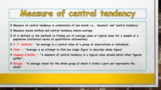
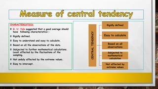
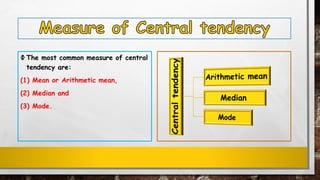
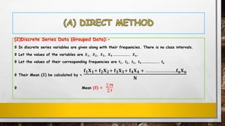
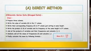
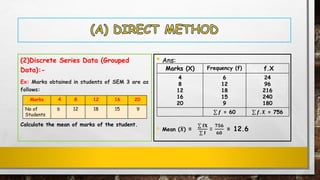
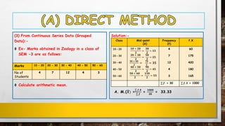
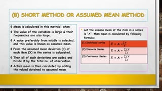
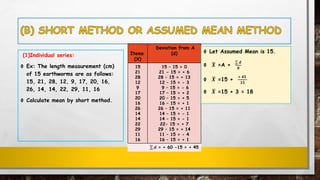
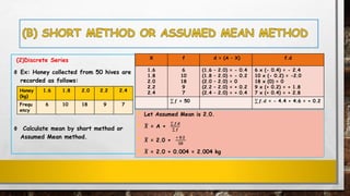
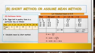
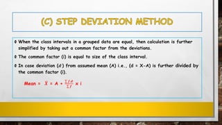
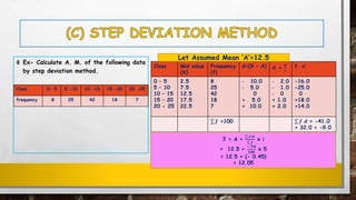
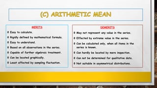
The document discusses various measures of central tendency and methods to calculate the arithmetic mean. It defines central tendency as a single value that describes a typical or average value in a data set. The three most common measures of central tendency are the mean, median, and mode. The document outlines different methods to calculate the arithmetic mean, including the direct method, short method, and step deviation method. It provides examples and step-by-step calculations for each method.

2. Ф A measure of central tendency is a single value
that describes a typical in a set of data as a
whole.
Ф In general term, it is the average of items in a
series.
Ф It is just the center of the data of distribution.
Ф It does not provide information about the
individual data.
Ф It gives overall picture about the concentration
of values in the central part of items in a series.
Measuring height of student in a class

3. Ф Measure of central tendency is combination of two words i.e., ‘measure’ and ‘central tendency’.
Ф Measure means method and central tendency means average.
Ф It is defined as the methods to finding out of average value or typical value for a sample or a
population (statistical series of quantitative information).
Ф J. P. Guilford:- “an average is a central value of a group of observations or individuals.
Ф Clark :- “Average is an attempt to find one single figure to describe whole figure”.
Ф Simpson & Kafka :- “A measure of central tendency is a typical value around which other figures
gather”.
Ф Waugh:- “A average stand for the whole group of which it forms a part yet represents the
whole”.

4. CHARACTERISTICS:
Ф G. U. Yule suggested that a good average should
have following characteristics:-
Ф Rigidly defined.
Ф Easy to understand and easy to calculate.
Ф Based on all the observations of the data.
Ф Subjected to further mathematical calculations.
Least affected by the fluctuations of the
sampling.
Ф Not unduly affected by the extreme values.
Ф Easy to intercept.
CENTRALTENDENCY
Rigidly defined
Easy to calculate
Based on all
observations
Subjected to
mathematical
calculation
Not affected by
extreme values

5. USES OF CENTRAL TENDENCY
i. It provides the overall picture of the series. Each and every figure can not be
remembered.
ii. It provides a clear picture about the field under study and necessary for conclusion.
iii. It gives a concise description of the performance of the group as a whole.
iv. It enables us to compare two or more groups in terms of typical performance.

6. Ф The most common measure of central
tendency are:
(1) Mean or Arithmetic mean,
(2) Median and
(3) Mode.

7. Ф “Arithmetic mean” or “mean” is the term used for average.
Ф It is common measure of central tendency of observation.
Ф It may be calculated by several formulae.
Ф It has been defined as “the quotient obtained by dividing the total of the values of
a variable by the total number of their observations or items”.
Ф H. E. Grant (1935) defines “The arithmetic mean or simply mean is the sum of the
separate scores or measures divided by their number”.

8. Arithmetic Mean can be calculated
by following methods.
Ф These are :-
A. Direct Method or Long Method
B. Short Method or Assumed Mean
Method and
C. Step Deviation Method
Arithmetic
Mean
Direct
Method
Short
Method
Step Deviation
Method

9. (1)Individual Series Data (Raw Data):-
In this method mean is calculated directly by following steps:
Ф Place all the variables of the Data.
Ф Sum together all the variables.
Ф Divide this total by the number of observations.
Ф Let the values of the variables are 𝑿 𝟏, 𝑿 𝟐, 𝑿 𝟑, 𝑿 𝟒……………….. 𝑿 𝒏
Ф The number of observations is N,
Ф Mean (ഥ𝑿) =
𝐒𝐮𝐦 𝐨𝐟 𝐚𝐥𝐥 𝐭𝐡𝐞 𝐯𝐚𝐫𝐢𝐚𝐛𝐥𝐞𝐬
𝐍𝐮𝐦𝐛𝐞𝐫 𝐨𝐟 𝐎𝐛𝐬𝐞𝐫𝐯𝐚𝐭𝐢𝐨𝐧𝐬
=
σ 𝑿 𝟏+ 𝑿 𝟐+ 𝑿 𝟑+ 𝑿 𝟒………………..+ 𝑿 𝒏
𝐍
=
σ𝒊=𝟏
𝒏
𝑿 𝒊
𝒏
=
σ 𝑿
𝒏

10. (1) Individual series data (Raw data):-
Ф Ex:- Marks obtained in internal
examination in zoology by 10 students
are as follows:- 30, 48, 36, 67, 43, 54,
17, 42, 05, 68. Find out the mean of
marks of students.
Ans :
Ф Mean (ഥ𝑿) =
σ 𝑿
𝒏
Ф =
𝟑𝟎+𝟒𝟖+𝟑𝟔+𝟔𝟕+𝟒𝟑+𝟓𝟒+𝟏𝟕+𝟒𝟐+𝟎𝟓+𝟔𝟖
𝟏𝟎
Ф or =
𝟒𝟏𝟎
𝟏𝟎
Ф = 41

11. (2)Discrete Series Data (Grouped Data):-
Ф In discrete series variables are given along with their frequencies. There is no class intervals.
Ф Let the values of the variables are 𝑿 𝟏, 𝑿 𝟐, 𝑿 𝟑, 𝑿 𝟒……………….. 𝑿 𝒏.
Ф Let the values of their corresponding frequencies are 𝐟 𝟏, 𝐟 𝟐, 𝐟 𝟑, 𝐟 𝟒……………….. 𝐟 𝐧
Ф Their Mean (ഥ𝑿) be calculated by =
𝐟 𝟏 𝐗 𝟏+ 𝐟 𝟐 𝐗 𝟐+ 𝐟 𝟑 𝐗 𝟑+ 𝐟 𝟒 𝐗 𝟒 + …………………….𝐟 𝐧 𝐗 𝐧
𝐍
Ф Mean (ഥ𝑿) =
σ 𝐟𝐗
σ 𝐟

12. (2)Discrete Series Data (Grouped Data):-
Steps:-
Ф Prepare three columns.
Ф Write the value of variable (X) in the 1st column.
Ф Write their corresponding frequency (f) in 2nd column just setting in same height.
Ф Write the product (f.X) of variable and its frequency at the same height in 3rd column.
Ф Add all the products of variables and their frequencies and calculate σ 𝒇. 𝑿
Ф Similarly add all the values of frequencies (f) and calculate σ 𝒇.
Ф Finally calculate the mean by following formula:- Mean (ഥ𝑿) =
σ 𝐟𝐗
σ 𝐟

13. (2)Discrete Series Data (Grouped
Data):-
Ex: Marks obtained in students of SEM 3 are as
follows:
Calculate the mean of marks of the student.
• Ans:
• Mean (ഥ𝑿) =
σ 𝐟𝐗
σ 𝐟
=
𝟕𝟓𝟔
𝟔𝟎
= 12.6
Marks 4 8 12 16 20
No of
Students
6 12 18 15 9
Marks (X) Frequency (f) f.X
4
8
12
16
20
6
12
18
15
9
24
96
216
240
180
σ 𝒇 = 60 σ 𝒇. 𝑿 = 756

14. (3) From Continuous Series Data (Grouped Data):-
Ф In continuous series data, variables are groups in classes of equal size and each class is continuous with its
preceding and next class group.
Steps:
Ф Four columns are prepared
Ф Write class size in 1st column.
Ф Write the mid point (X) of each class in 2nd column (by adding the lowest and highest values and dividing by two).
Ф Write the frequency (f) of each class in same sequence or height in 3rd column.
Ф Multiply the mid point (X) of each class with its frequency (f) and write the product fX in 4th column.
Ф Calculate mean by the formula - (ഥ𝑿) =
σ 𝐟𝐗
σ 𝐟

15. (3) From Continuous Series Data (Grouped
Data):-
Ф Ex- Marks obtained in Zoology in a class of
SEM -3 are as follows:
Ф Calculate arithmetic mean.
Marks 10 - 20 20 - 30 30 - 40 40 - 50 50 - 60
No of
Students
4 7 12 4 3
Solution:-
A. M.(ഥ𝑿) =
σ 𝒇.𝑿
σ 𝒇
=
𝟏𝟎𝟎𝟎
𝟑𝟎
= 33.33
Class Mid-point
(X)
Frequency
(f)
f.X
10 – 20
20 – 30
30 – 40
40 – 50
50 – 60
𝟏𝟎 + 𝟐𝟎
𝟐
=
𝟑𝟎
𝟐
= 𝟏𝟓
𝟐𝟎 + 𝟑𝟎
𝟐
=
𝟓𝟎
𝟐
= 𝟐𝟓
𝟑𝟎 + 𝟒𝟎
𝟐
=
𝟕𝟎
𝟐
= 𝟑𝟓
𝟒𝟎 + 𝟓𝟎
𝟐
=
𝟗𝟎
𝟐
= 𝟒𝟓
𝟓𝟎 + 𝟔𝟎
𝟐
=
𝟏𝟏𝟎
𝟐
= 𝟓𝟓
4
7
12
4
3
60
175
420
180
165
σ 𝒇 = 30 σ 𝒇. 𝑿 = 1000

16. Ф Mean is calculated in this method, when
Ф The value of the variables is large & their
frequencies are also large.
Ф A value preferably from middle is selected,
and this value is known as assumed mean.
Ф From the assumed mean deviation (d) of
each item (X) in the series is calculated.
Ф Then all of such deviations are added and
Divide it by the total no. of observation.
Ф Actual mean is then calculated by adding
the valued obtained to assumed mean
• Let the assume mean of the item in a series
is “A”, then mean is calculated by following
formula:
(1) Individual series ഥ𝑿 = A +
σ 𝒅
𝑵
(2) Discrete Series ഥ𝑿 = A +
σ 𝒇.𝒅
σ 𝒇
(3) Continuous Series ഥ𝑿 = A +
σ 𝒇.𝒅
σ 𝒇

17. (1)Individual series:
Ф Ex: The length measurement (cm)
of 15 earthworms are as follows:
15, 21, 28, 12, 9, 17, 20, 16,
26, 14, 14, 22, 29, 11, 16
Ф Calculate mean by short method.
Items
(X)
Deviation from A
(d)
15
21
28
12
9
17
20
16
26
14
14
22
29
11
16
15 – 15 = 0
21 - 15 = + 6
28 – 15 = + 13
12 – 15 = - 3
9 – 15 = - 6
17 – 15 = + 2
20 – 15 = + 5
16 – 15 = + 1
26 – 15 = + 11
14 – 15 = - 1
14 – 15 = - 1
22- 15 = + 7
29 – 15 = + 14
11 – 15 = - 4
16 – 15 = + 1
σ 𝒅 = + 60 -15 = + 45
Ф Let Assumed Mean is 15.
Ф ഥ𝑿 =A +
σ 𝒅
𝑵
Ф ഥ𝑿 =15 +
+ 𝟒𝟓
𝟏𝟓
Ф ഥ𝑿 =15 + 3 = 18

18. (2)Discrete Series
Ф Ex: Honey collected from 50 hives are
recorded as follows:
Ф Calculate mean by short method or
Assumed Mean method.
• Let Assumed Mean is 2.0.
• ഥ𝑿 = A +
σ 𝒇.𝒅
σ 𝒇
• ഥ𝑿 = 2.0 +
+ 𝟎.𝟐
𝟓𝟎
• ഥ𝑿 = 2.0 + 0.004 = 2.004 kg
Honey
(kg)
1.6 1.8 2.0 2.2 2.4
Frequ
ency
6 10 18 9 7
X f d = (A – X) f.d
1.6
1.8
2.0
2.2
2.4
6
10
18
9
7
(1.6 – 2.0) = - 0.4
(1.8 – 2.0) = - 0.2
(2.0 – 2.0) = 0
(2.2 – 2.0) = + 0.2
(2.4 – 2.0) = + 0.4
6 x (- 0.4) = - 2.4
10 x (- 0.2) = -2.0
18 x (0) = 0
9 x (+ 0.2) = + 1.8
7 x (+ 0.4) = + 2.8
σ 𝒇 = 50 σ 𝒇. 𝒅 = - 4.4 + 4.6 = + 0.2

19. • (3) Continuous Series
Ф Ex: Eggs laid in poultry farm in a
particular day as follows:
Ф Calculate mean by short method. ഥ𝑿 =A +
σ 𝒇.𝒅
σ 𝒇
• ഥ𝑿 = 12.5 + (
+ 𝟓.𝟎
𝟓𝟎
)
• ഥ𝑿 = 12.5 + 0.1 = 12.6
Class 0 - 5 5 - 10 10 -15 15- 20 20 -25
Freque
ncy
6 10 18 9 7
Class Mid point (f) d = (A –X) f.d
0 – 5
5 – 10
10 – 15
15 – 20
20 – 25
2.5
7.5
12.5
17.5
22.5
6
10
18
9
7
- 10.0
- 5.0
0
+ 5.0
+ 10.0
- 60.0
- 50.0
0
+ 45.0
+ 70.0
σ 𝒇 = 50 σ 𝒇. 𝒅 = -110 +
115 = + 5.0
Let Assumed mean is 12.5

20. Ф When the class intervals in a grouped data are equal, then calculation is further
simplified by taking out a common factor from the deviations.
Ф The common factor (i) is equal to size of the class interval.
Ф In case deviation (𝒅,
) from assumed mean (A) i.e., (d = X-A) is further divided by
the common factor (i).
Mean = ഥ𝑿 = A +
σ 𝒇.𝒅,
σ 𝒇
x i

21. Ф Ex- Calculate A. M. of the following data
by step deviation method.
Class 0- 5 5 -10 10 -15 15 -20 20 -25
frequency 8 25 42 18 7
Class Mid value
(X)
Frequency
(f)
d=(X – A) 𝒅,
=
𝒅
𝒊
f. 𝒅,
0 – 5
5 – 10
10 – 15
15 – 20
20 - 25
2.5
7.5
12.5
17.5
22.5
8
25
42
18
7
- 10.0
- 5.0
0
+ 5.0
+ 10.0
- 2.0
- 1.0
- 0
+ 1.0
+ 2.0
-16.0
-25.0
0
+18.0
+14.0
σ 𝒇 =100 σ 𝒇. 𝒅,
= -41.0
+ 32.0 = -9.0
Let Assumed Mean ‘A’=12.5
ഥ𝑿 = A +
σ 𝒇.𝒅,
σ 𝒇
x i
= 12.5 +
− 𝟗.𝟎
𝟏𝟎𝟎
x 5
= 12.5 + (- 0.45)
= 12.05

22. • If the mean ഥ𝒙 𝟏 & ഥ𝒙 𝟐 and the size 𝒏 𝟏 & 𝒏 𝟐 are two sets of a single
distribution, then the combined mean for resultant sets in the distribution can
be calculated by the formula:-
• Combined Mean: ഥ𝑿 =
𝐧 𝟏ത𝐱 𝟏+𝐧 𝟐ത𝐱 𝟐
𝐧 𝟏+𝐧 𝟐

23. Ex- There are 60 students in Zoology Core in SEM 3 in a College, of which 25 are
girls and rest are boys. If the mean marks obtained by girls 42 and mean marks of
the boys are 40. find out the mean marks of all 60 students.
Ans: the no. of girls (𝒏 𝟏)= 25, mean marks ഥ𝒙 𝟏 =42
the no. of boys (𝒏 𝟐) = (60 – 25) = 35, mean marks ഥ𝒙 𝟐 = 40
• Combined Mean: ഥ𝑿 =
𝐧 𝟏ത𝐱 𝟏+𝐧 𝟐ത𝐱 𝟐
𝐧 𝟏+𝐧 𝟐
=
𝟐𝟓 𝒙 𝟒𝟐 +𝟑𝟓 𝒙 𝟒𝟎
𝟐𝟓+𝟑𝟓
=
𝟏𝟎𝟓𝟎+𝟏𝟒𝟎𝟎
𝟔𝟎
• ഥ𝑿 =
𝟐𝟒𝟓𝟎
𝟔𝟎
= 40.83

24. MERITS
Ф Easy to calculate.
Ф Rigidly defined by mathematical formula.
Ф Easy to understand.
Ф Based on all observations in the series.
Ф Capable of further algebraic treatment.
Ф Can be located graphically.
Ф Least affected by sampling fluctuation.
DEMERITS
Ф May not represent any value in the series.
Ф Effected by extreme value in the series.
Ф Can be calculated only, when all items in the
series is known.
Ф Can hardly be located by mere inspection.
Ф Can not be determined for qualitative data.
Ф Not suitable in asymmetrical distributions.