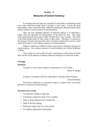
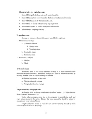
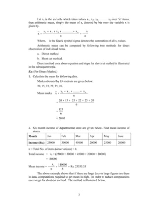
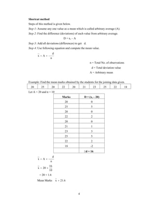
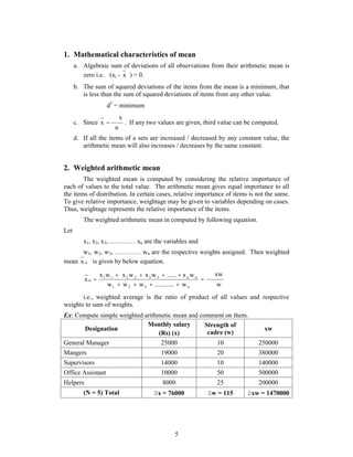
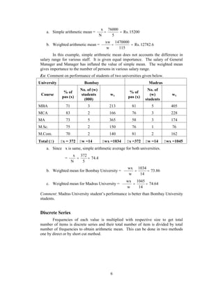
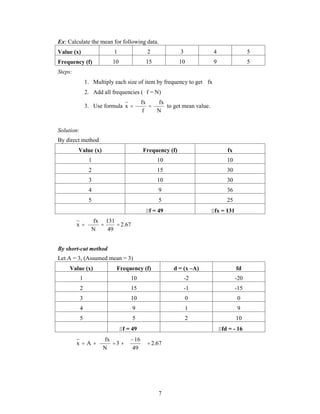
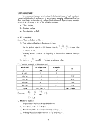
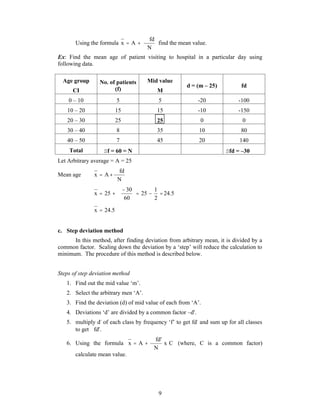
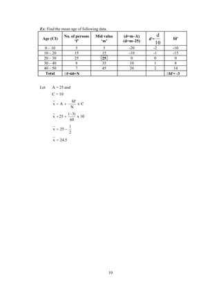
This document discusses measures of central tendency and different methods for calculating averages. It begins by defining central tendency as a single value that represents the characteristics of an entire data set. Three common measures of central tendency are introduced: the mean, median, and mode. The document then focuses on explaining how to calculate the arithmetic mean, or average, including the direct method, shortcut method, and how it applies to discrete and continuous data series. Weighted averages are also covered. In summary, the document provides an overview of key concepts in measures of central tendency and how to calculate various types of averages.

1. Session – 4
Measures of Central Tendency
A classified statistical data may sometimes be described as distributed around
some value called the central value or average is some sense. It gives the most
representative value of the entire data. Different methods give different central values
and are referred to as the measures of central tendency.
Thus, the most important objective of statistical analysis is to determine a
single value that represents the characteristics of the entire raw data. This single
value representing the entire data is called ‘Central value’ or an ‘average’. This value
is the point around which all other values of data cluster. Therefore, it is known as
the measure of location and since this value is located at central point nearest to other
values of the data it is also called as measures of central tendency.
Different methods give different central values and are referred as measures of
central tendency. The common measures of central tendency are a) Mean b) Median
c) Mode.
These values are very useful not only in presenting overall picture of entire
data, but also for the purpose of making comparison among two or more sets of data.
1
Average
Definition
Average is a value which is typical or representative of a set of data.
- Murry R. Speigal
Average is an attempt to find one single figure to describe whole of figures.
- Clark & Sekkade
From above definitions it is clear that average is a typical value of the entire
data and is a measure of central tendency.
Functions of an average
 To represents complex or large data.
 It facilitates comparative study of two variables.
 Helps to study population from sample data.
 Helps in decision making.
 Represents single value for a series of data.
 To establish mathematical relationship.

2. Characteristics of a typical average
 It should be rigidly defined and easily understandable.
 It should be simple to compute and in the form of mathematical formula.
 It should be based on all the items in the data.
 It should not be unduly influenced by any single item.
 It should be capable of further mathematical treatment.
 It should have sampling stability.
2
Types of average
Average or measures of central tendency are of following types.
1. Mathematical average
a. Arithmetical mean
i. Simple mean
ii. Weighted mean
b. Geometric mean
c. Harmonic mean
2. Positional Averages
a. Median
b. Mode
Arithmetic mean
Arithmetic mean is also called arithmetic average. It is most commonly used
measures of central tendency. Arithmetic average of a series is the value obtained by
dividing the total value of various item by its number.
Arithmetic average are of two types
a. Simple arithmetic average
b. Weighted arithmetic average
Simple arithmetic average (Mean)
Arithmetic mean is simply sometimes referred as ‘Mean’. Ex: Mean income,
Mean expenses, Mean marks etc.
Unlike other averages, mean has to be computed by considering each and
every observations in the series. Hence, the mean cannot be found by either by
inspection or observation of items.
Simple arithmetic mean is equal to sum of the variable divided by their
number of observations in the sample.

3. Let xi is the variable which takes values x1, x2, x3,……… xn over ‘n’ items,
then arithmetic mean, simply the mean of x, denoted by bar over the variable x is
given by.
x 1 2 3 n  

x  x  ......... 
x
x 1 2 n 20  15  23  22  25  20

3
n
x
   
x x x ............... x
n

Where,  is the Greek symbol sigma denotes the summation of all xi values.
Arithmetic mean can be computed by following two methods for direct
observation of individual items.
a. Direct method
b. Short cut method.
Direct method uses above equation and steps for short cut method is illustrated
in the subsequent topic.
Ex: (For Direct Method)
1. Calculate the mean for following data.
Marks obtained by 65 students are given below:
20, 15, 23, 22, 25, 20.
Mean marks
n
6
125 
6
= 20.83
2. Six month income of departmental store are given below. Find mean income of
stores.
Month Jan Feb Mar Apr May June
Income (Rs.) 25000 30000 45000 20000 25000 20000
n = Total No. of items (observations) = 6
Total income = xi = (25000 + 30000 + 45000 + 20000 + 20000)
= 140000

xi  140000
 Mean income = Rs. 23333.33
6
n
The above example shows that if there are large data or large figures are there
in data, computations required to get mean in high. In order to reduce computations
one can go for short-cut method. The method is illustrated below.

4. Shortcut method
Steps of this method is given below.
Step 1: Assume any one value as a mean which is called arbitrary average (A).
Step 2: Find the difference (deviations) of each value from arbitrary average.
4
D = xi – A
Step 3: Add all deviations (differences) to get d.
Step 4: Use following equation and compute the mean value.
n
d
x A   
n = Total No. of observations
d = Total deviation value
A = Arbitrary mean
Example: Find the mean marks obtained by the students for the joining data given.
20 25 20 22 20 21 23 25 22 18
Let A = 20 and n = 10
Marks D = (xi – 20)
20 0
25 5
20 0
22 2
20 0
21 1
23 3
25 5
22 2
18 -2
d = 16
n
d
x A   
16
10
x  20 
= 20 + 1.6
Mean Marks x  21.6

5. 1. Mathematical characteristics of mean
a. Algebraic sum of deviations of all observations from their arithmetic mean is
x   . If any two values are given, third value can be computed.
   
x w x w x w ...... x w
1 1 2 2 3 3 n n
5
zero i.e. (xi - x ) = 0.
b. The sum of squared deviations of the items from the mean is a minimum, that
is less than the sum of squared deviations of items from any other value.
d2 = minimum
c. Since
n
x
d. If all the items of a sets are increased / decreased by any constant value, the
arithmetic mean will also increases / decreases by the same constant.
2. Weighted arithmetic mean
The weighted mean is computed by considering the relative importance of
each of values to the total value. The arithmetic mean gives equal importance to all
the items of distribution. In certain cases, relative importance of items is not the same.
To give relative importance, weightage may be given to variables depending on cases.
Thus, weightage represents the relative importance of the items.
The weighted arithmetic mean in computed by following equation.
Let
x1, x2, x3, ………… xn are the variables and
w1, w2, w3, ………… wn are the respective weights assigned. Then weighted
mean x w is given by below equation.
 
xw

   

w
w w w ............ w
x
1 2 3 n
w
i.e., weighted average is the ratio of product of all values and respective
weights to sum of weights.
Ex: Compute simple weighted arithmetic mean and comment on them.
Designation
Monthly salary
(Rs) (x)
Strength of
cadre (w) xw
General Manager 25000 10 250000
Mangers 19000 20 380000
Supervisors 14000 10 140000
Office Assistant 10000 50 500000
Helpers 8000 25 200000
(N = 5) Total x = 76000 w = 115 xw = 1470000

6. x  76000


a. Simple arithmetic mean = Rs. 15200
5
xw  

6
N
1470000
b. Weighted arithmetic mean = Rs. 12782.6
115
w

In this example, simple arithmetic mean does not accounts the difference in
salary range for various staff. It is given equal importance. The salary of General
Manager and Manager has inflated the value of simple mean. The weighted mean
gives importance to the number of persons in various salary range.
Ex: Comment on performance of students of two universities given below.
University Bombay Madras
Course
% of
pas (x)
No. of (w)
students
(000)
wx
% of
pas (x)
No. of
(w)
students
wx
MBA 71 3 213 81 5 405
MCA 83 2 166 76 3 228
MA 73 5 365 58 3 174
M.Sc. 75 2 150 76 1 76
M.Com. 70 2 140 81 2 162
Total () x = 372 w =14 wx =1034 x =372 w =14 wx =1045
a. Since x is same, simple arithmetic average for both universities.
x  372


= 74.4
5
N
wx  1034


b. Weighted mean for Bombay University = 73.86
14
w

wx  1045


c. Weighted mean for Madras University = 74.64
14
w

Comment: Madras University student’s performance is better than Bombay University
students.
Discrete Series
Frequencies of each value is multiplied with respective size to get total
number of items is discrete series and their total number of item is divided by total
number of frequencies to obtain arithmetic mean. This can be done in two methods
one by direct or by short cut method.

7. Ex: Calculate the mean for following data.
Value (x) 1 2 3 4 5
Frequency (f) 10 15 10 9 5
Steps:
1. Multiply each size of item by frequency to get fx
2. Add all frequencies (f = N)

 fx
to get mean value.
7
3. Use formula
N
fx
f
x



Solution:
By direct method
Value (x) Frequency (f) fx
1 10 10
2 15 30
3 10 30
4 9 36
5 5 25
f = 49 fx = 131
2.67
131


x  
49
fx
N
By short-cut method
Let A = 3, (Assumed mean = 3)
Value (x) Frequency (f) d = (x –A) fd
1 10 -2 -20
2 15 -1 -15
3 10 0 0
4 9 1 9
5 5 2 10
f = 49 fd = - 16
2.67
16
 

x A 3
 49
fx
N


 

 

8. 8
Continuous series
In continuous frequency distribution, the individual value of each item in the
frequency distribution is not known. In a continuous series the mid points of various
class intervals are written down to replace the class interval. In continuous series the
mean can be calculated by any of the following methods.
a. Direct method
b. Short cut method
c. Step deviation method
a. Direct method
Steps of their method are as follows
1. Find out the mid value of class group or class.

23 30  50

Ex: For a class interval 20-30, the mid value is 25
2
2
mid value
is denoted by ‘m’.
2. Multiply the mid value ‘m’ by frequency ‘f’ of each class and sum up to get
fm.
3. Use
fm
N
x

 where N = f formula to get mean value.
Ex: Compute the mean for following data.
Age group
(CI)
No. of persons
(f)
Mid point
‘m’
fm
0 – 10 5 5 25
10 – 20 15 15 225
20 – 30 25 25 625
30 – 40 8 35 280
40 – 50 7 45 315
Total f = 60 = N fm = 1470
fm fm
 1470


Mean age = 245
60
N
f



x = 24.5
b. Short cut method
Steps of above methods are described below.
1. Find the mid value of each class
2. Assume any of the mid value as arbitrary average (A).
3. Multiply the deviation (differences) ‘d’ by frequency ‘f’.

9.  
25 x    
fd'
9
Using the formula
fd
N
x A

  find the mean value.
Ex: Find the mean age of patient visiting to hospital in a particular day using
following data.
Age group
CI
No. of patients
(f)
Mid value
M
d = (m – 25) fd
0 – 10 5 5 -20 -100
10 – 20 15 15 -10 -150
20 – 30 25 25 0 0
30 – 40 8 35 10 80
40 – 50 7 45 20 140
Total f = 60 = N fd = –30
Let Arbitrary average = A = 25
Mean age
fd
N
x A

 
24.5
1
2
25
30
60


 
x  24.5
c. Step deviation method
In this method, after finding deviation from arbitrary mean, it is divided by a
common factor. Scaling down the deviation by a ‘step’ will reduce the calculation to
minimum. The procedure of this method is described below.
Steps of step deviation method
1. Find out the mid value ‘m’.
2. Select the arbitrary men ‘A’.
3. Find the deviation (d) of mid value of each from ‘A’.
4. Deviations ‘d’ are divided by a common factor –d'.
5. multiply d' of each class by frequency ‘f’ to get fd' and sum up for all classes
to get fd'.
6. Using the formula x C
N
x A

  (where, C is a common factor)
calculate mean value.

10. 10
Ex: Find the mean age of following data.
Age (CI) No. of persons
‘f’
Mid value
‘m’
(d=m–A)
(d=m–25) d'=
d
10
fd'
0 – 10 5 5 -20 -2 -10
10 – 20 15 15 -10 -1 -15
20 – 30 25 25 0 0 0
30 – 40 8 35 10 1 8
40 – 50 7 45 20 2 14
Total f=60=N fd'= -3
Let A = 25 and
C = 10
x C
fd'
N
x A

 
x 10
( 3)
60
x 25

 
1
2
x  25 
x  24.5