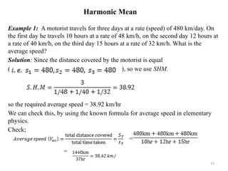
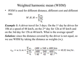
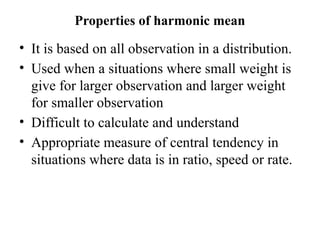
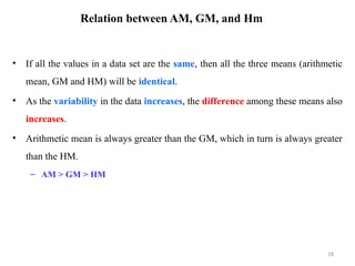
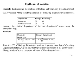
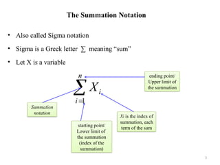
2. Summarizing of Data
• A measure of central tendency is a descriptive statistic that describes the
average, or typical value of a set of scores.
• It is also defined as a single value that is used to describe “center” of the
data
1
Typical value
(Center of data)
2.1 Measures of Central Tendency
2.2 Types of measures of central tendency
• Good properties of typical average
– Computation should be based on all the observed values.
– It should be simple to understand and easy to interpret.
– As little as affected by fluctuations of sampling.
– should not unduly be influenced by extreme values.
– it should be defined rigidly which means that it should have a definite value
• There are three common measures of central tendency
– Mean
– Median
– Mode
2
The Summation Notation
• Also called Sigma notation
• Sigma is a Greek letter ∑ meaning “sum”
• Let X is a variable
3


n
i
i
X
1
starting point/
Lower limit of
the summation
(index of the
summation)
Summation
notation
Xi is the index of
summation, each
term of the sum
ending point/
Upper limit of
the summation
The Summation Notation..
• Properties of summation notation
4
n
n
i
i
n
i
i
n
n
i
i
n
n
n
i
i
i
n
n
i
i
CX
CX
CX
X
C
CX
X
X
X
X
Y
X
Y
X
Y
X
Y
X
X
X
X
X






























2
1
1
1
2
2
2
2
1
1
2
2
2
1
1
1
2
1
1
The Mean
• Mean is the most commonly used measure of central tendency. There are
different types of mean
– Arithmetic mean,
– Weighted mean,
– Geometric mean (GM) and
– Harmonic mean (HM)
• If mentioned without an adjective (as mean), it generally refers to the
arithmetic mean.
5
The Arithmetic Mean
• It is computed by adding all the values in the data set divided by the number
of observations in it.
• If we have the raw data, mean is given by the formula
• If we have frequency distribution (ungrouped) mean is given by the formula
• If we have frequency distribution (grouped) mean is given by the formula
LCB/UCB is lower/upper class boundary
6
n
X
X
n
i
i


 1
n
X
f
X
n
i
i
i


 1
2
,
1 i
i
i
n
i
i
i
UCB
LCB
m
where
n
m
f
X





The Arithmetic Mean …
• Example 1: The following data is the weight (in Kg) of eight youths:
32,37,41,39,36,43,48 and 36. Calculate the arithmetic mean of their weight.
(Ans:312/8=39 )
• Example 2: The ages of a random sample of patients in a given hospital in Ethiopia is
given below: (Ans: 16.075)
7
Age (xi) Number of patients (fi)
10 3
12 6
14 10
16 14
18 11
20 5
22 4
The Arithmetic Mean …
• Example 3: Age in year of 20 women who attended health education at Jimma Health
center in 1986 is summarized in the table. What is the mean age of these women. (Ans:
670/20=33.5)
8
Time (in seconds) Number of students
23-26 3
27-30 4
31-34 3
35-38 5
39-42 5
Properties of Arithmetic Mean …
• It can be computed for any set of numerical data, it always exists, and unique.
• It depends on all observations.
• The sum of deviations of the observations about the mean is zero i.e.
• It is greatly affected by extreme values.
• It lends itself to further statistical treatment, for instance, combinations of means.
• It is relatively reliable, i.e. it is not greatly affected by fluctuations in sampling.
• The sum of squares of deviations of all observations about the mean is the minimum
• If a constant is added to all observations, the new mean is old mean plus constant
• If all observations are multiplied by a constant, the new mean is the multiple of the constant and old
mean
• If wrong value is recorded and latter on it is discovered, the new corrected mean is
9
 
n
X
X
X
X
wrong
corr
wrong
corr



Weighted Mean
• Weighted mean is calculated when certain values in a data set are more
important than the others.
• A weight wi is attached to each of the values xi to reflect this importance.
• The weighted mean is computed as
• Example: CGPA of a students (each result is weighted by credit of a course) [Ans:
2.88]
10




 k
i
i
k
i
i
i
w
w
x
w
X
1
1
Geometric Mean
• It is defined as the arithmetic mean of the values taken on a log scale.
• It is also expressed as the nth
root of the product of an observation.
• GM is an appropriate measure when values change exponentially and in case of
skewed distribution that can be made symmetrical by a log transformation.
• Note: The geometric mean is useful in finding the average of percentages,
ratios, indexes, or growth rates.
• One important disadvantage of GM is that it cannot be used if any of the values
are zero or negative.
11
Geometric Mean…
Example 1:- The G.M of 4, 8 and 6 is.
Solution:
Example 2: The man gets three annual raises in his salary. At the end of first year,
he gets an increase of 4%, at the end of the second year, he gets an increase of 6%
and at the end of the third year, he gets an increase of 9% of his salary. What is the
average percentage increase in the three periods?
Solution:
12
Properties of geometric mean
– Its calculations are not as such easy.
– It involves all observations during computation
– It may not be defined even it a single observation
is negative.
– If the value of one observation is zero its values
becomes zero.
Harmonic Mean
• Another important mean is the harmonic mean, which is suitable measure of
central tendency when the data pertains to speed, rates and price.
• It is the reciprocal of the arithmetic mean of the observations.
• Let be n variant values in a set of observations, then simple
harmonic mean is given by:
• Note: SHM is used for equal distances, equal costs and equal rates.
14
Harmonic Mean
Example 1: A motorist travels for three days at a rate (speed) of 480 km/day. On
the first day he travels 10 hours at a rate of 48 km/h, on the second day 12 hours at
a rate of 40 km/h, on the third day 15 hours at a rate of 32 km/h. What is the
average speed?
Solution: Since the distance covered by the motorist is equal
( ), so we use SHM.
so the required average speed = 38.92 km/hr
We can check this, by using the known formula for average speed in elementary
physics.
Check;
=
=
15
Weighted harmonic mean (WHM)
• WHM is used for different distance, different cost and different
rate.
Example 1: A driver travel for 3 days. On the 1st
day he drives for
10h at a speed of 48 km/h, on the 2nd
day for 12h at 45 km/h and
on the 3rd day for 15h at 40 km/h. What is the average speed?
Solution: since the distance covered by the driver is not equal, so
we use WHM by taking the distance as weights (wi).
Properties of harmonic mean
• It is based on all observation in a distribution.
• Used when a situations where small weight is
give for larger observation and larger weight
for smaller observation
• Difficult to calculate and understand
• Appropriate measure of central tendency in
situations where data is in ratio, speed or rate.
Relation between AM, GM, and Hm
• If all the values in a data set are the same, then all the three means (arithmetic
mean, GM and HM) will be identical.
• As the variability in the data increases, the difference among these means also
increases.
• Arithmetic mean is always greater than the GM, which in turn is always greater
than the HM.
– AM > GM > HM
18
Median
• If the sample data are arranged in increasing order, the median is
– if n is an odd number, median is middle value
• Example: systolic blood pressure of seven persons were given as 113, 124, 124, 132,
146, 151, and 170. what is the median systolic blood pressure? (Ans: 132)
– if n is an even number, midway between the two middle values
• Six men with high cholesterol participated in a study to investigate the effects of diet on
cholesterol level. At the beginning of the study, their cholesterol levels (mg/dL) were as
follows:366, 327, 274, 292, 274 and 230. what is the median cholesterol level?
(Ans:283)
19
Median …
– If the data is in ungrouped frequency distribution, median is the class with largest
less than cumulative frequency smaller than or equal to half of the total observation
• Example: Forty five students were taken to field and evaluated their performance using 60m
pure speed test. The time is recorded in seconds, and the result is summarized in the table. What
is the median performance of these students. (Ans: 19 secs)
20
Time (in
seconds)
Number of
students
Less than
cumulative
frequency
15 4 4
16 9 13
18 8 21
19 14 35
20 10 45
Median …
– If the data is in grouped frequency distribution, median is
• Example: fifty students were taken to field and evaluated their performance using 100 m
pure speed test. The time is recorded in seconds, and the result is summarized in the table.
What is the median performance of these students. (Ans: 20.81 secs)
21
Time (in seconds) Number of students
14-16 6
17-19 12
20-22 16
23-25 9
26-28 7
Mode
• The most frequent observation (value) in a data
• An observation with the largest frequency
• There can be no mode Eg: 25, 27, 22, 18
• There can be only one mode-unimodal Eg: 25, 27, 22, 25,18
• There can be two mode-bimodal Eg: 25, 27, 22, 27, 25, 18, 20
• There can be more than two mode-multimodal Eg: 25, 27, 22, 27, 25, 18, 20, 19, 22, 17
• Mode grouped frequency distribution
• f1 = frequency of the modal class
• f0 = frequency of the class preceding the modal class
• f2 = frequency of the class next to the modal class
22
Mode…
• The most frequent observation (value) in a data
– Example: Twenty five amateur cyclists were taken to field and their time is
recorded to complete a given distance. The time is recorded in seconds, and
the result is summarized in the table. What is the modal time to complete the
distance. (Ans: 29.5 secs)
23
Time (in seconds) Number of
Atheletes
15.5- 21.5 3
21.5-27.5 6
27.5-33.5 8
33.5-39.5 4
39.5-45.5 3
45.5-51.5 1
2.3 Quantiles
• Quartiles are three points which divide an array into four parts in
such a way that each portion contains an equal number of
elements.
– First quartile (Q1) 25% of the observations lies below or equal to it
– Second quartile (Q2) 50 % of the observations lies below or equal to it and
– Third quartile (Q3) 75% of the observations lies below or equal to it
• The ith
quartile for raw data is
• If there is an even number of data items, then we need to get the average
of the middle numbers. 24
 
4
1


n
i
Qi
Quantiles
• Example: Find the median, lower quartile and upper quartile of the
following numbers.
a) 12, 5, 22, 30, 7, 36, 14, 42, 15, 53, 25
b) 12, 5, 22, 30, 7, 36, 14, 42, 15, 53, 25, 65
• Solution: first arrange data from smallest to largest
a)
b)
25
13 23.5 39
Quantiles
• The ith
quartile for grouped frequency distribution is
26
Quantiles …
• Deciles are nine points which divide an array into 10 parts in such
a way that each part contains equal number of elements.
– The nine deciles are denoted by D1, D2, …, D9
– First decile (D1) 10% of the observations lies below or equal to it
– Second decile (D2) 20% of the observations lies below or equal to it etc
• The ith
decile for grouped frequency distribution is
27
Quantiles …
• Percentiles are 99 points which divide an array into 100 parts in
such a way that each part consists of equal number of elements.
– The ninty nine percentiles are denoted by P1, P2, …, P99
– First percentile (P1) 1% of the observations lies below or equal to it
– Second percentile (P2) 2% of the observations lies below or equal to it etc
• The ith
percentile for grouped frequency distribution is
28
Quantiles …
– Example:- The following frequency distribution is the score of 25 students.
Compute the following
quantities
● First quartile (Ans:44.92)
●Ninth decile (Ans:65.75)
●forty fifth percentile (Ans:51.38)
Remark:
29
Score Number
of
students
25-29 1
30-34 1
35-39 1
40-44 3
45-49 3
50-54 6
55-59 4
60-64 3
65-69 2
70-74 1
90
9
20
2
10
1
75
3
50
5
2
25
1
;
;
; P
D
P
D
P
D
P
Q
Median
P
D
Q
P
Q









2.4 Measures of Dispersion
30
Introduction
– Central tendency measures do not reveal the variability present in the data.
– Dispersion is the scatteredness of the data series around it average.
– Dispersion is the extent to which values in a distribution differ from the
average of the distribution
– A measure of statistical dispersion is a nonnegative real number that is zero
if all the data are the same and increases as the data become more diverse.
• Why we need measures of dispersion?
– Determine the reliability of an average
– Serve as a basis for the control of the variability
– To compare the variability of two or more series and
– Facilitate the use of other statistical measures.
31
Introduction…
• Properties of a good measures of dispersion
– It should be rigidly defined
– It should be easy to understand and to calculate
– It should be based on all observations of data
– It should be easily subjected to further mathematical treatment
– It should be least affected by sampling fluctuation
– It shouldn’t be unduly affected by extreme values
32
Introduction…
• There are many types of dispersion measures
– Range /Relative Range (Coefficient of range)
– Inter Quartile Range/ coefficient of quartile deviation
– Mean Absolute Deviation /Coefficient of mean deviation
– Variance/Standard Deviation/ coefficient of variation
• Measures of dispersion cane be absolute or relative.
– When measurements are observed with different units, or have different
averages use relative measures of dispersion.
33
Range (R)
• Range is the difference between two extreme values in a data
• Denoted by R
R = max − min
• Only two values are used in its calculation.
• It is influenced by an extreme value (non-robust).
• It is easy to compute and understand.
34
Properties of range
• It is the simplest crude measure and can be easily
understood
• It takes into account only two values which causes it
to be a poor measure of dispersion
• Very sensitive to extreme observations
• The larger the sample size, the larger the range
Inter Quartile Range
• Measures the range of the middle 50% of the values only
• Is defined as the difference between the upper and lower quartiles
• Interquartile range = upper quartile - lower quartile
= Q3 - Q1
• The semi-interquartile range (or SIR) is defined as the difference of
the first and third quartiles divided by two
SIR = (Q3 - Q1) / 2
• The SIR is often used with skewed data as it is insensitive to the extreme
scores
36
Properties of IQR
• It is a simple and versatile measure
• It encloses the central 50% of the observations
• It is not based on all observations but only on two
specific values
• Since it excludes the lowest and highest 25% values, it
is not affected by extreme values
• Less sensitive to the size of the sample
Variance
• Variance is the mean of squared deviation of observations from
their arithmetic mean
– All values are used in the calculation.
– It is not extremely influenced by outliers.
– The units of variance are awkward: the square of the original
units.
• Therefore standard deviation is more natural since it recovers the original units.
38
𝑃
𝑜𝑝𝑢𝑙𝑎𝑡𝑖𝑜𝑛 𝑣𝑎𝑟𝑖𝑎𝑛𝑐𝑒 = 𝜎2
=
σ ሺ
𝑥𝑖 − 𝜇ሻ
2
𝑁
𝑖=1
𝑁
→𝑓𝑜𝑟𝑝𝑜𝑝𝑢𝑙𝑎𝑡𝑖𝑜𝑛.
𝑆
𝑎𝑚𝑝𝑙𝑒𝑣𝑎𝑟𝑖𝑎𝑛𝑐
𝑒= 𝑠2
=
σ ሺ
𝑥
𝑖 − 𝑥
ҧ
ሻ
2
𝑛
𝑖=1
𝑛 − 1
→𝑓
𝑜𝑟𝑠𝑎𝑚𝑝𝑙𝑒.
• In general, the sample variance is computed
by:
𝑠2
=
‫ە‬
ۖ
ۖ
‫۔‬
ۖ
ۖ
‫ۓ‬
σ ሺ
𝑥𝑖 − 𝑥
ҧ
ሻ
2
𝑛
𝑖=1
𝑛 − 1
=
σ 𝑥𝑖
2
− 𝑛𝑥
ҧ
2
𝑛
𝑖=1
𝑛− 1
. →𝑓𝑜𝑟 𝑟𝑎𝑤𝑑𝑎𝑡𝑎.
σ 𝑓
𝑖ሺ
𝑥𝑖 − 𝑥
ҧ
ሻ
2
𝑘
𝑖=1
σ 𝑓
𝑖
𝑘
𝑖=1 − 1
=
σ 𝑓
𝑖𝑥𝑖
2
− 𝑛𝑥
ҧ
2
𝑘
𝑖=1
𝑛− 1
. →𝑓𝑜𝑟𝑢𝑛𝑔𝑟𝑜𝑢𝑝𝑒𝑑𝑑𝑎𝑡𝑎.
σ 𝑓
𝑖ሺ
𝑚𝑖 − 𝑥
ҧ
ሻ
2
𝑘
𝑖=1
σ 𝑓
𝑖
𝑘
𝑖=1 − 1
=
σ 𝑓
𝑖𝑚𝑖
2
− 𝑛𝑥
ҧ
2
𝑘
𝑖=1
𝑛 − 1
. →𝑓𝑜𝑟𝑔𝑟𝑜𝑢𝑝𝑒𝑑𝑑𝑎𝑡𝑎.
Standard Deviation
• One of the most useful measures of dispersion is the standard deviation.
• It is based on deviations from the mean of the data.
• The sample standard deviation is found by calculating the square root of
the variance.
• To calculate standard deviation follow this step
1. Calculate the mean of the numbers
2. Find the deviations from the mean.
3. Square each deviation
4. Sum the squared deviations
5. Divide the sum in Step 4 by n – 1
6. Take the square root of the quotient in Step 5
40
2
( )
.
1
x x
s
n




Example 1: Compute the variance for the sample: 5, 14, 2, 2 and
17.
Solution:
Example 2: Suppose the data given below indicates time in
minute required for a laboratory experiment to compute a certain
laboratory test. Calculate the mean, variance and standard
deviation for the following data.
𝑛 = 5, ෍ 𝑥𝑖 = 40,
𝑛
𝑖=1
𝑥
ҧ
= 8, ෍ 𝑥𝑖
2
𝑛
𝑖=1
= 518.
𝑠2
=
σ 𝑥𝑖
2
− 𝑛𝑥
ҧ
2
𝑛
𝑖=1
𝑛− 1
=
518− 5𝑥82
5− 1
= 49.5. , 𝑆= ξ49.5 = 7.04.
32 36 40 44 48 Total
2 5 8 4 1 20
64 180 320 176 48 788
2048 6480 12800 7744 2304 31376
𝑥
ҧ
= 39.4, 𝑠2
=
31376− 20𝑥ሺ
39.4ሻ
2
19
= 17.31. , 𝑆= ξ17.31 = 4.16.
Properties of Variance
• The variance is always non-negative ( ).
• If every element of the data is multiplied by a
constant "c", then the new variance
• When a constant is added to all elements of the
data, then the variance does not change.
• The variance of a constant (c) measured in n
times is zero. i.e. (var(c) = 0).
𝑠2
𝑛𝑒𝑤 = 𝑐2
𝑥𝑠2
𝑜𝑙𝑑.
𝑠2
≥ 0
Coefficient of Variation
• The Coefficient of Variation (CV) for a data set defined as the ratio of the standard
deviation to the mean
• It shows the extent of variability in relation to mean of the population.
• It is a normalized measure of dispersion of a probability distribution or frequency
distribution.
– All values are used in the calculation.
– The actual value of the CV is independent of the unit in which the measurement has been
taken, so it is a dimensionless number.
– For comparison between data sets with different units or widely different means, one
should use the coefficient of variation instead of the standard deviation.
43
%
100


x
s
CV
Coefficient of Variation
Example: Last semester, the students of Biology and Chemistry Departments took
Stat 273 course. At the end of the semester, the following information was recorded.
Compare the relative dispersions of the two departments’ scores using the
appropriate way.
Solution:
Since the CV of Biology Department students is greater than that of Chemistry
Department students, we can say that there is more dispersion in the distribution of
Biology students’ scores compared with that of Chemistry students.
44
Department Biology Chemistry
Mean score 79 64
Standard deviation 23 11
Chemistry
Department
Biology Department
23
100 29.11%
79
CV   
11
100 17.19%
64
CV   
2.5 Standard Score
• If X is a measurement from a distribution with mean and standard
deviation S, then its value in standard units is
• Z gives the deviations from the mean in units of standard deviation
• Z gives the number of standard deviation a particular observation lie
above or below the mean.
• It is used to compare two observations coming from different groups
45
X
S
X
X
Z


Standard Score
• Example: Two groups of people were trained to perform a certain task
and tested to find out which group is faster to learn the task. For the two
groups the following information was given:
Value Group one Group two
Mean 10.4 min 11.9 min
Stan.dev. 1.2 min 1.3 min
• Relatively speaking:
a) Which group is more consistent in its performance? (Ans: Group 2)
b) Suppose a person A from group one take 9.2 minutes while person B from Group
two take 9.3 minutes, who was faster in performing the task? Why? (Ans: person B
is faster)
46
00
.
1
2
.
1
4
.
10
2
.
9
1
1






S
x
x
Z A
00
.
2
3
.
1
9
.
11
3
.
9
2
2






S
x
x
Z B
Coefficient of variation for group 1:
Z-score of Person B:
Z-score of Person A:
%
54
.
11
%
100
4
.
10
2
.
1
%
100
1
1





x
S
CV
Coefficient of variation for group 2: %
92
.
10
%
100
9
.
11
3
.
1
%
100
2
2





x
S
CV
CV for group 2 < CV for group 1 group 2 is more consistent
Z-score of Person B < Z-score of Person A  Person B is faster than
person A
Solution

Introduction to Measurement CHAPTER 2 (2) (1).pptx

  • 1.
    2. Summarizing ofData • A measure of central tendency is a descriptive statistic that describes the average, or typical value of a set of scores. • It is also defined as a single value that is used to describe “center” of the data 1 Typical value (Center of data) 2.1 Measures of Central Tendency
  • 2.
    2.2 Types ofmeasures of central tendency • Good properties of typical average – Computation should be based on all the observed values. – It should be simple to understand and easy to interpret. – As little as affected by fluctuations of sampling. – should not unduly be influenced by extreme values. – it should be defined rigidly which means that it should have a definite value • There are three common measures of central tendency – Mean – Median – Mode 2
  • 3.
    The Summation Notation •Also called Sigma notation • Sigma is a Greek letter ∑ meaning “sum” • Let X is a variable 3   n i i X 1 starting point/ Lower limit of the summation (index of the summation) Summation notation Xi is the index of summation, each term of the sum ending point/ Upper limit of the summation
  • 4.
    The Summation Notation.. •Properties of summation notation 4 n n i i n i i n n i i n n n i i i n n i i CX CX CX X C CX X X X X Y X Y X Y X Y X X X X X                               2 1 1 1 2 2 2 2 1 1 2 2 2 1 1 1 2 1 1
  • 5.
    The Mean • Meanis the most commonly used measure of central tendency. There are different types of mean – Arithmetic mean, – Weighted mean, – Geometric mean (GM) and – Harmonic mean (HM) • If mentioned without an adjective (as mean), it generally refers to the arithmetic mean. 5
  • 6.
    The Arithmetic Mean •It is computed by adding all the values in the data set divided by the number of observations in it. • If we have the raw data, mean is given by the formula • If we have frequency distribution (ungrouped) mean is given by the formula • If we have frequency distribution (grouped) mean is given by the formula LCB/UCB is lower/upper class boundary 6 n X X n i i    1 n X f X n i i i    1 2 , 1 i i i n i i i UCB LCB m where n m f X     
  • 7.
    The Arithmetic Mean… • Example 1: The following data is the weight (in Kg) of eight youths: 32,37,41,39,36,43,48 and 36. Calculate the arithmetic mean of their weight. (Ans:312/8=39 ) • Example 2: The ages of a random sample of patients in a given hospital in Ethiopia is given below: (Ans: 16.075) 7 Age (xi) Number of patients (fi) 10 3 12 6 14 10 16 14 18 11 20 5 22 4
  • 8.
    The Arithmetic Mean… • Example 3: Age in year of 20 women who attended health education at Jimma Health center in 1986 is summarized in the table. What is the mean age of these women. (Ans: 670/20=33.5) 8 Time (in seconds) Number of students 23-26 3 27-30 4 31-34 3 35-38 5 39-42 5
  • 9.
    Properties of ArithmeticMean … • It can be computed for any set of numerical data, it always exists, and unique. • It depends on all observations. • The sum of deviations of the observations about the mean is zero i.e. • It is greatly affected by extreme values. • It lends itself to further statistical treatment, for instance, combinations of means. • It is relatively reliable, i.e. it is not greatly affected by fluctuations in sampling. • The sum of squares of deviations of all observations about the mean is the minimum • If a constant is added to all observations, the new mean is old mean plus constant • If all observations are multiplied by a constant, the new mean is the multiple of the constant and old mean • If wrong value is recorded and latter on it is discovered, the new corrected mean is 9   n X X X X wrong corr wrong corr   
  • 10.
    Weighted Mean • Weightedmean is calculated when certain values in a data set are more important than the others. • A weight wi is attached to each of the values xi to reflect this importance. • The weighted mean is computed as • Example: CGPA of a students (each result is weighted by credit of a course) [Ans: 2.88] 10      k i i k i i i w w x w X 1 1
  • 11.
    Geometric Mean • Itis defined as the arithmetic mean of the values taken on a log scale. • It is also expressed as the nth root of the product of an observation. • GM is an appropriate measure when values change exponentially and in case of skewed distribution that can be made symmetrical by a log transformation. • Note: The geometric mean is useful in finding the average of percentages, ratios, indexes, or growth rates. • One important disadvantage of GM is that it cannot be used if any of the values are zero or negative. 11
  • 12.
    Geometric Mean… Example 1:-The G.M of 4, 8 and 6 is. Solution: Example 2: The man gets three annual raises in his salary. At the end of first year, he gets an increase of 4%, at the end of the second year, he gets an increase of 6% and at the end of the third year, he gets an increase of 9% of his salary. What is the average percentage increase in the three periods? Solution: 12
  • 13.
    Properties of geometricmean – Its calculations are not as such easy. – It involves all observations during computation – It may not be defined even it a single observation is negative. – If the value of one observation is zero its values becomes zero.
  • 14.
    Harmonic Mean • Anotherimportant mean is the harmonic mean, which is suitable measure of central tendency when the data pertains to speed, rates and price. • It is the reciprocal of the arithmetic mean of the observations. • Let be n variant values in a set of observations, then simple harmonic mean is given by: • Note: SHM is used for equal distances, equal costs and equal rates. 14
  • 15.
    Harmonic Mean Example 1:A motorist travels for three days at a rate (speed) of 480 km/day. On the first day he travels 10 hours at a rate of 48 km/h, on the second day 12 hours at a rate of 40 km/h, on the third day 15 hours at a rate of 32 km/h. What is the average speed? Solution: Since the distance covered by the motorist is equal ( ), so we use SHM. so the required average speed = 38.92 km/hr We can check this, by using the known formula for average speed in elementary physics. Check; = = 15
  • 16.
    Weighted harmonic mean(WHM) • WHM is used for different distance, different cost and different rate. Example 1: A driver travel for 3 days. On the 1st day he drives for 10h at a speed of 48 km/h, on the 2nd day for 12h at 45 km/h and on the 3rd day for 15h at 40 km/h. What is the average speed? Solution: since the distance covered by the driver is not equal, so we use WHM by taking the distance as weights (wi).
  • 17.
    Properties of harmonicmean • It is based on all observation in a distribution. • Used when a situations where small weight is give for larger observation and larger weight for smaller observation • Difficult to calculate and understand • Appropriate measure of central tendency in situations where data is in ratio, speed or rate.
  • 18.
    Relation between AM,GM, and Hm • If all the values in a data set are the same, then all the three means (arithmetic mean, GM and HM) will be identical. • As the variability in the data increases, the difference among these means also increases. • Arithmetic mean is always greater than the GM, which in turn is always greater than the HM. – AM > GM > HM 18
  • 19.
    Median • If thesample data are arranged in increasing order, the median is – if n is an odd number, median is middle value • Example: systolic blood pressure of seven persons were given as 113, 124, 124, 132, 146, 151, and 170. what is the median systolic blood pressure? (Ans: 132) – if n is an even number, midway between the two middle values • Six men with high cholesterol participated in a study to investigate the effects of diet on cholesterol level. At the beginning of the study, their cholesterol levels (mg/dL) were as follows:366, 327, 274, 292, 274 and 230. what is the median cholesterol level? (Ans:283) 19
  • 20.
    Median … – Ifthe data is in ungrouped frequency distribution, median is the class with largest less than cumulative frequency smaller than or equal to half of the total observation • Example: Forty five students were taken to field and evaluated their performance using 60m pure speed test. The time is recorded in seconds, and the result is summarized in the table. What is the median performance of these students. (Ans: 19 secs) 20 Time (in seconds) Number of students Less than cumulative frequency 15 4 4 16 9 13 18 8 21 19 14 35 20 10 45
  • 21.
    Median … – Ifthe data is in grouped frequency distribution, median is • Example: fifty students were taken to field and evaluated their performance using 100 m pure speed test. The time is recorded in seconds, and the result is summarized in the table. What is the median performance of these students. (Ans: 20.81 secs) 21 Time (in seconds) Number of students 14-16 6 17-19 12 20-22 16 23-25 9 26-28 7
  • 22.
    Mode • The mostfrequent observation (value) in a data • An observation with the largest frequency • There can be no mode Eg: 25, 27, 22, 18 • There can be only one mode-unimodal Eg: 25, 27, 22, 25,18 • There can be two mode-bimodal Eg: 25, 27, 22, 27, 25, 18, 20 • There can be more than two mode-multimodal Eg: 25, 27, 22, 27, 25, 18, 20, 19, 22, 17 • Mode grouped frequency distribution • f1 = frequency of the modal class • f0 = frequency of the class preceding the modal class • f2 = frequency of the class next to the modal class 22
  • 23.
    Mode… • The mostfrequent observation (value) in a data – Example: Twenty five amateur cyclists were taken to field and their time is recorded to complete a given distance. The time is recorded in seconds, and the result is summarized in the table. What is the modal time to complete the distance. (Ans: 29.5 secs) 23 Time (in seconds) Number of Atheletes 15.5- 21.5 3 21.5-27.5 6 27.5-33.5 8 33.5-39.5 4 39.5-45.5 3 45.5-51.5 1
  • 24.
    2.3 Quantiles • Quartilesare three points which divide an array into four parts in such a way that each portion contains an equal number of elements. – First quartile (Q1) 25% of the observations lies below or equal to it – Second quartile (Q2) 50 % of the observations lies below or equal to it and – Third quartile (Q3) 75% of the observations lies below or equal to it • The ith quartile for raw data is • If there is an even number of data items, then we need to get the average of the middle numbers. 24   4 1   n i Qi
  • 25.
    Quantiles • Example: Findthe median, lower quartile and upper quartile of the following numbers. a) 12, 5, 22, 30, 7, 36, 14, 42, 15, 53, 25 b) 12, 5, 22, 30, 7, 36, 14, 42, 15, 53, 25, 65 • Solution: first arrange data from smallest to largest a) b) 25 13 23.5 39
  • 26.
    Quantiles • The ith quartilefor grouped frequency distribution is 26
  • 27.
    Quantiles … • Decilesare nine points which divide an array into 10 parts in such a way that each part contains equal number of elements. – The nine deciles are denoted by D1, D2, …, D9 – First decile (D1) 10% of the observations lies below or equal to it – Second decile (D2) 20% of the observations lies below or equal to it etc • The ith decile for grouped frequency distribution is 27
  • 28.
    Quantiles … • Percentilesare 99 points which divide an array into 100 parts in such a way that each part consists of equal number of elements. – The ninty nine percentiles are denoted by P1, P2, …, P99 – First percentile (P1) 1% of the observations lies below or equal to it – Second percentile (P2) 2% of the observations lies below or equal to it etc • The ith percentile for grouped frequency distribution is 28
  • 29.
    Quantiles … – Example:-The following frequency distribution is the score of 25 students. Compute the following quantities ● First quartile (Ans:44.92) ●Ninth decile (Ans:65.75) ●forty fifth percentile (Ans:51.38) Remark: 29 Score Number of students 25-29 1 30-34 1 35-39 1 40-44 3 45-49 3 50-54 6 55-59 4 60-64 3 65-69 2 70-74 1 90 9 20 2 10 1 75 3 50 5 2 25 1 ; ; ; P D P D P D P Q Median P D Q P Q         
  • 30.
    2.4 Measures ofDispersion 30
  • 31.
    Introduction – Central tendencymeasures do not reveal the variability present in the data. – Dispersion is the scatteredness of the data series around it average. – Dispersion is the extent to which values in a distribution differ from the average of the distribution – A measure of statistical dispersion is a nonnegative real number that is zero if all the data are the same and increases as the data become more diverse. • Why we need measures of dispersion? – Determine the reliability of an average – Serve as a basis for the control of the variability – To compare the variability of two or more series and – Facilitate the use of other statistical measures. 31
  • 32.
    Introduction… • Properties ofa good measures of dispersion – It should be rigidly defined – It should be easy to understand and to calculate – It should be based on all observations of data – It should be easily subjected to further mathematical treatment – It should be least affected by sampling fluctuation – It shouldn’t be unduly affected by extreme values 32
  • 33.
    Introduction… • There aremany types of dispersion measures – Range /Relative Range (Coefficient of range) – Inter Quartile Range/ coefficient of quartile deviation – Mean Absolute Deviation /Coefficient of mean deviation – Variance/Standard Deviation/ coefficient of variation • Measures of dispersion cane be absolute or relative. – When measurements are observed with different units, or have different averages use relative measures of dispersion. 33
  • 34.
    Range (R) • Rangeis the difference between two extreme values in a data • Denoted by R R = max − min • Only two values are used in its calculation. • It is influenced by an extreme value (non-robust). • It is easy to compute and understand. 34
  • 35.
    Properties of range •It is the simplest crude measure and can be easily understood • It takes into account only two values which causes it to be a poor measure of dispersion • Very sensitive to extreme observations • The larger the sample size, the larger the range
  • 36.
    Inter Quartile Range •Measures the range of the middle 50% of the values only • Is defined as the difference between the upper and lower quartiles • Interquartile range = upper quartile - lower quartile = Q3 - Q1 • The semi-interquartile range (or SIR) is defined as the difference of the first and third quartiles divided by two SIR = (Q3 - Q1) / 2 • The SIR is often used with skewed data as it is insensitive to the extreme scores 36
  • 37.
    Properties of IQR •It is a simple and versatile measure • It encloses the central 50% of the observations • It is not based on all observations but only on two specific values • Since it excludes the lowest and highest 25% values, it is not affected by extreme values • Less sensitive to the size of the sample
  • 38.
    Variance • Variance isthe mean of squared deviation of observations from their arithmetic mean – All values are used in the calculation. – It is not extremely influenced by outliers. – The units of variance are awkward: the square of the original units. • Therefore standard deviation is more natural since it recovers the original units. 38 𝑃 𝑜𝑝𝑢𝑙𝑎𝑡𝑖𝑜𝑛 𝑣𝑎𝑟𝑖𝑎𝑛𝑐𝑒 = 𝜎2 = σ ሺ 𝑥𝑖 − 𝜇ሻ 2 𝑁 𝑖=1 𝑁 →𝑓𝑜𝑟𝑝𝑜𝑝𝑢𝑙𝑎𝑡𝑖𝑜𝑛. 𝑆 𝑎𝑚𝑝𝑙𝑒𝑣𝑎𝑟𝑖𝑎𝑛𝑐 𝑒= 𝑠2 = σ ሺ 𝑥 𝑖 − 𝑥 ҧ ሻ 2 𝑛 𝑖=1 𝑛 − 1 →𝑓 𝑜𝑟𝑠𝑎𝑚𝑝𝑙𝑒.
  • 39.
    • In general,the sample variance is computed by: 𝑠2 = ‫ە‬ ۖ ۖ ‫۔‬ ۖ ۖ ‫ۓ‬ σ ሺ 𝑥𝑖 − 𝑥 ҧ ሻ 2 𝑛 𝑖=1 𝑛 − 1 = σ 𝑥𝑖 2 − 𝑛𝑥 ҧ 2 𝑛 𝑖=1 𝑛− 1 . →𝑓𝑜𝑟 𝑟𝑎𝑤𝑑𝑎𝑡𝑎. σ 𝑓 𝑖ሺ 𝑥𝑖 − 𝑥 ҧ ሻ 2 𝑘 𝑖=1 σ 𝑓 𝑖 𝑘 𝑖=1 − 1 = σ 𝑓 𝑖𝑥𝑖 2 − 𝑛𝑥 ҧ 2 𝑘 𝑖=1 𝑛− 1 . →𝑓𝑜𝑟𝑢𝑛𝑔𝑟𝑜𝑢𝑝𝑒𝑑𝑑𝑎𝑡𝑎. σ 𝑓 𝑖ሺ 𝑚𝑖 − 𝑥 ҧ ሻ 2 𝑘 𝑖=1 σ 𝑓 𝑖 𝑘 𝑖=1 − 1 = σ 𝑓 𝑖𝑚𝑖 2 − 𝑛𝑥 ҧ 2 𝑘 𝑖=1 𝑛 − 1 . →𝑓𝑜𝑟𝑔𝑟𝑜𝑢𝑝𝑒𝑑𝑑𝑎𝑡𝑎.
  • 40.
    Standard Deviation • Oneof the most useful measures of dispersion is the standard deviation. • It is based on deviations from the mean of the data. • The sample standard deviation is found by calculating the square root of the variance. • To calculate standard deviation follow this step 1. Calculate the mean of the numbers 2. Find the deviations from the mean. 3. Square each deviation 4. Sum the squared deviations 5. Divide the sum in Step 4 by n – 1 6. Take the square root of the quotient in Step 5 40 2 ( ) . 1 x x s n    
  • 41.
    Example 1: Computethe variance for the sample: 5, 14, 2, 2 and 17. Solution: Example 2: Suppose the data given below indicates time in minute required for a laboratory experiment to compute a certain laboratory test. Calculate the mean, variance and standard deviation for the following data. 𝑛 = 5, ෍ 𝑥𝑖 = 40, 𝑛 𝑖=1 𝑥 ҧ = 8, ෍ 𝑥𝑖 2 𝑛 𝑖=1 = 518. 𝑠2 = σ 𝑥𝑖 2 − 𝑛𝑥 ҧ 2 𝑛 𝑖=1 𝑛− 1 = 518− 5𝑥82 5− 1 = 49.5. , 𝑆= ξ49.5 = 7.04. 32 36 40 44 48 Total 2 5 8 4 1 20 64 180 320 176 48 788 2048 6480 12800 7744 2304 31376 𝑥 ҧ = 39.4, 𝑠2 = 31376− 20𝑥ሺ 39.4ሻ 2 19 = 17.31. , 𝑆= ξ17.31 = 4.16.
  • 42.
    Properties of Variance •The variance is always non-negative ( ). • If every element of the data is multiplied by a constant "c", then the new variance • When a constant is added to all elements of the data, then the variance does not change. • The variance of a constant (c) measured in n times is zero. i.e. (var(c) = 0). 𝑠2 𝑛𝑒𝑤 = 𝑐2 𝑥𝑠2 𝑜𝑙𝑑. 𝑠2 ≥ 0
  • 43.
    Coefficient of Variation •The Coefficient of Variation (CV) for a data set defined as the ratio of the standard deviation to the mean • It shows the extent of variability in relation to mean of the population. • It is a normalized measure of dispersion of a probability distribution or frequency distribution. – All values are used in the calculation. – The actual value of the CV is independent of the unit in which the measurement has been taken, so it is a dimensionless number. – For comparison between data sets with different units or widely different means, one should use the coefficient of variation instead of the standard deviation. 43 % 100   x s CV
  • 44.
    Coefficient of Variation Example:Last semester, the students of Biology and Chemistry Departments took Stat 273 course. At the end of the semester, the following information was recorded. Compare the relative dispersions of the two departments’ scores using the appropriate way. Solution: Since the CV of Biology Department students is greater than that of Chemistry Department students, we can say that there is more dispersion in the distribution of Biology students’ scores compared with that of Chemistry students. 44 Department Biology Chemistry Mean score 79 64 Standard deviation 23 11 Chemistry Department Biology Department 23 100 29.11% 79 CV    11 100 17.19% 64 CV   
  • 45.
    2.5 Standard Score •If X is a measurement from a distribution with mean and standard deviation S, then its value in standard units is • Z gives the deviations from the mean in units of standard deviation • Z gives the number of standard deviation a particular observation lie above or below the mean. • It is used to compare two observations coming from different groups 45 X S X X Z  
  • 46.
    Standard Score • Example:Two groups of people were trained to perform a certain task and tested to find out which group is faster to learn the task. For the two groups the following information was given: Value Group one Group two Mean 10.4 min 11.9 min Stan.dev. 1.2 min 1.3 min • Relatively speaking: a) Which group is more consistent in its performance? (Ans: Group 2) b) Suppose a person A from group one take 9.2 minutes while person B from Group two take 9.3 minutes, who was faster in performing the task? Why? (Ans: person B is faster) 46
  • 47.
    00 . 1 2 . 1 4 . 10 2 . 9 1 1       S x x Z A 00 . 2 3 . 1 9 . 11 3 . 9 2 2       S x x Z B Coefficientof variation for group 1: Z-score of Person B: Z-score of Person A: % 54 . 11 % 100 4 . 10 2 . 1 % 100 1 1      x S CV Coefficient of variation for group 2: % 92 . 10 % 100 9 . 11 3 . 1 % 100 2 2      x S CV CV for group 2 < CV for group 1 group 2 is more consistent Z-score of Person B < Z-score of Person A  Person B is faster than person A Solution