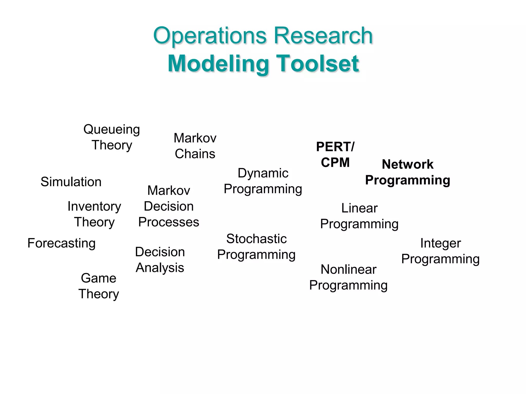
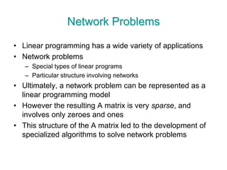
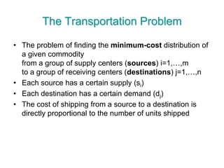
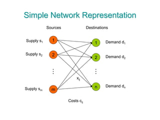
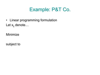
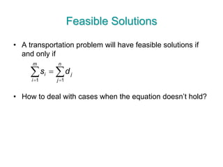
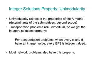
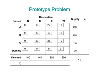
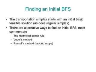
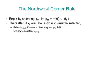
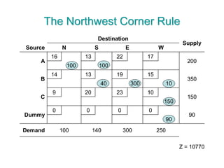
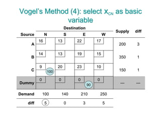
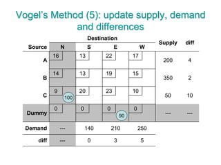
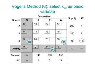
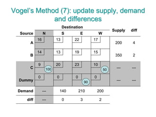
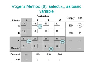
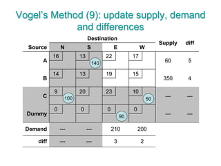
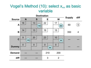
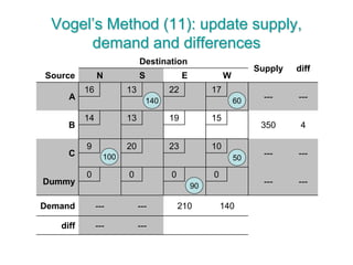
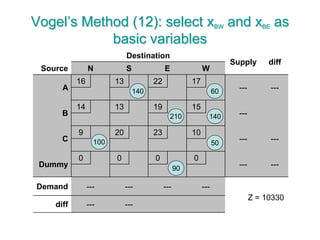
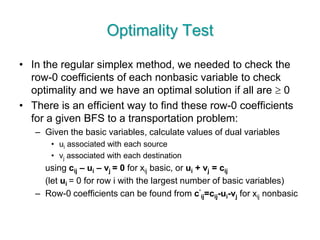
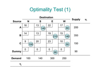
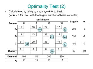
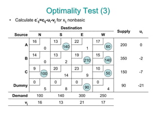
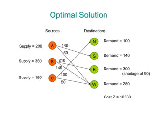
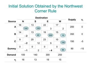
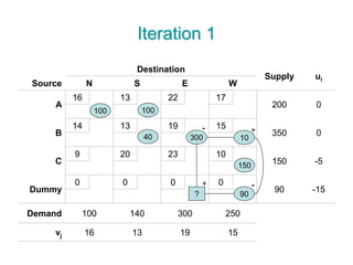
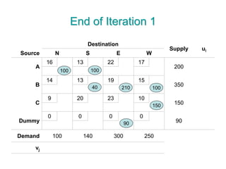
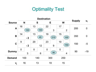
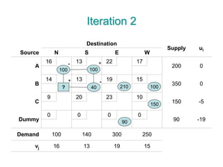
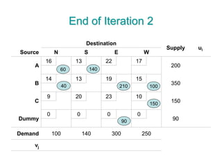
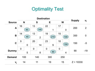
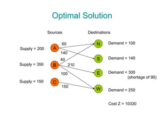
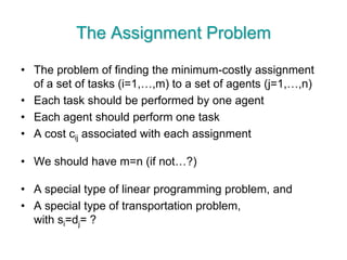
The document discusses operations research modeling tools, particularly focusing on linear programming and its application to network problems, including transportation and assignment problems. It explains the transportation problem, which aims to minimize distribution costs while satisfying supply and demand constraints, and introduces the transportation simplex method for finding optimal solutions. Several methods for finding initial basic feasible solutions, as well as optimization techniques within the context of transportation, are also outlined.

1. Operations Research
Modeling Toolset
Linear
Programming
Network
Programming
PERT/
CPM
Dynamic
Programming
Integer
Programming
Nonlinear
Programming
Game
Theory
Decision
Analysis
Markov
Chains
Queueing
Theory
Inventory
Theory
Forecasting
Markov
Decision
Processes
Simulation
Stochastic
Programming

2. Network Problems
• Linear programming has a wide variety of applications
• Network problems
– Special types of linear programs
– Particular structure involving networks
• Ultimately, a network problem can be represented as a
linear programming model
• However the resulting A matrix is very sparse, and
involves only zeroes and ones
• This structure of the A matrix led to the development of
specialized algorithms to solve network problems

3. Types of Network Problems
• Shortest Path
Special case: Project Management with PERT/CPM
• Minimum Spanning Tree
• Maximum Flow/Minimum Cut
• Minimum Cost Flow
Special case: Transportation and Assignment Problems
• Set Covering/Partitioning
• Traveling Salesperson
• Facility Location
and many more

4. The Transportation Problem

5. The Transportation Problem
• The problem of finding the minimum-cost distribution of
a given commodity
from a group of supply centers (sources) i=1,…,m
to a group of receiving centers (destinations) j=1,…,n
• Each source has a certain supply (si)
• Each destination has a certain demand (dj)
• The cost of shipping from a source to a destination is
directly proportional to the number of units shipped

6. Simple Network Representation
1
2
m
1
2
n
Sources Destinations
…
…
Supply s1
Supply s2
Supply sm
Demand d1
Demand d2
Demand dn
xij
Costs cij

7. Example: P&T Co.
• Produces canned peas at three canneries
Bellingham, WA, Eugene, OR, and Albert Lea, MN
• Ships by truck to four warehouses
Sacramento, CA, Salt Lake City, UT, Rapid City, SD, and
Albuquerque, NM
• Estimates of shipping costs, production capacities and
demands for the upcoming season is given
• The management needs to make a plan on the least
costly shipments to meet demand

8. Example: P&T Co. Map
1
2
3
1
2
3
4

9. Example: P&T Co. Data
Warehouse
Cannery 1 2 3 4
Supply
(Truckloads)
1 $ 464 $ 513 $ 654 $ 867 75
2 $ 352 $ 216 $ 690 $ 791 125
3 $ 995 $ 682 $ 388 $ 685 100
Demand
(Truckloads)
80 65 70 85
Shipping cost
per truckload

10. Example: P&T Co.
• Network representation

11. Example: P&T Co.
• Linear programming formulation
Let xij denote…
Minimize
subject to

12. General LP Formulation for Transportation
Problems

13. Feasible Solutions
• A transportation problem will have feasible solutions if
and only if
• How to deal with cases when the equation doesn’t hold?
 

n
j
j
m
i
i ds
11

14. Integer Solutions Property: Unimodularity
• Unimodularity relates to the properties of the A matrix
(determinants of the submatrices, beyond scope)
• Transportation problems are unimodular, so we get the
integers solutions property:
For transportation problems, when every si and dj
have an integer value, every BFS is integer valued.
• Most network problems also have this property.

15. Transportation Simplex Method
• Since any transportation problem can be formulated as
an LP, we can use the simplex method to find an optimal
solution
• Because of the special structure of a transportation LP,
the iterations of the simplex method have a very special
form
• The transportation simplex method is nothing but the
original simplex method, but it streamlines the iterations
given this special form

16. Transportation Simplex Method
Initialization
(Find initial CPF solution)
Is the
current
CPF
solution
optimal?
Move to a better
adjacent CPF solution
Stop
No
Yes

17. The Transportation Simplex Tableau
Destination
Supply ui
Source 1 2 … n
1
c11 c12
…
c1n
s1
2
c21 c22
…
c2n
s2
… … … … … …
m
cm1 cm2
…
cmn
sm
Demand d1 d2 … dn
Z =
vj

18. Prototype Problem
• Holiday shipments of iPods to distribution centers
• Production at 3 facilities,
– A, supply 200k
– B, supply 350k
– C, supply 150k
• Distribute to 4 centers,
– N, demand 100k
– S, demand 140k
– E, demand 300k
– W, demand 250k
• Total demand vs. total supply

19. Prototype Problem
Destination
Supply ui
Source N S E W
A
16 13 22 17
200
B
14 13 19 15
350
C
9 20 23 10
150
Dummy
0 0 0 0
90
Demand 100 140 300 250
Z =
vj

20. Finding an Initial BFS
• The transportation simplex starts with an initial basic
feasible solution (as does regular simplex)
• There are alternative ways to find an initial BFS, most
common are
– The Northwest corner rule
– Vogel’s method
– Russell’s method (beyond scope)

21. The Northwest Corner Rule
• Begin by selecting x11, let x11 = min{ s1, d1 }
• Thereafter, if xij was the last basic variable selected,
– Select xi(j+1) if source i has any supply left
– Otherwise, select x(i+1)j

22. The Northwest Corner Rule
Destination
Supply
Source N S E W
A
16 13 22 17
200
100 100
B
14 13 19 15
350
40 300 10
C
9 20 23 10
150
150
Dummy
0 0 0 0
90
90
Demand 100 140 300 250
Z = 10770

23. Vogel’s Method
• For each row and column, calculate its difference:
= (Second smallest cij in row/col) - (Smallest cij in row/col)
• For the row/col with the largest difference, select entry
with minimum cij as basic
• Eliminate any row/col with no supply/demand left from
further steps
• Repeat until BFS found

24. Vogel’s Method (1): calculate differences
Destination
Supply diff
Source N S E W
A
16 13 22 17
200 3
B
14 13 19 15
350 1
C
9 20 23 10
150 1
Dummy
0 0 0 0
90 0
Demand 100 140 300 250
diff 9 13 19 10

25. Vogel’s Method (2): select xDummyE as basic
variable
Destination
Supply diff
Source N S E W
A
16 13 22 17
200 3
B
14 13 19 15
350 1
C
9 20 23 10
150 1
Dummy
0 0 0 0
90 0
Demand 100 140 300 250
diff 9 13 19 10
90

26. Vogel’s Method (3): update supply, demand
and differences
Destination
Supply diff
Source N S E W
A
16 13 22 17
200 3
B
14 13 19 15
350 1
C
9 20 23 10
150 1
Dummy
0 0 0 0
--- ---
Demand 100 140 210 250
diff 5 0 3 5
90

27. Vogel’s Method (4): select xCN as basic
variable
Destination
Supply diff
Source N S E W
A
16 13 22 17
200 3
B
14 13 19 15
350 1
C
9 20 23 10
150 1
Dummy
0 0 0 0
--- ---
Demand 100 140 210 250
diff 5 0 3 5
90
100

28. Vogel’s Method (5): update supply, demand
and differences
Destination
Supply diff
Source N S E W
A
16 13 22 17
200 4
B
14 13 19 15
350 2
C
9 20 23 10
50 10
Dummy
0 0 0 0
--- ---
Demand --- 140 210 250
diff --- 0 3 5
90
100

29. Vogel’s Method (6): select xCW as basic
variable
Destination
Supply diff
Source N S E W
A
16 13 22 17
200 4
B
14 13 19 15
350 2
C
9 20 23 10
50 10
Dummy
0 0 0 0
--- ---
Demand --- 140 210 250
diff --- 0 3 5
90
100 50

30. Vogel’s Method (7): update supply, demand
and differences
Destination
Supply diff
Source N S E W
A
16 13 22 17
200 4
B
14 13 19 15
350 2
C
9 20 23 10
--- ---
Dummy
0 0 0 0
--- ---
Demand --- 140 210 200
diff --- 0 3 2
90
100 50

31. Vogel’s Method (8): select xAS as basic
variable
Destination
Supply diff
Source N S E W
A
16 13 22 17
200 4
B
14 13 19 15
350 2
C
9 20 23 10
--- ---
Dummy
0 0 0 0
--- ---
Demand --- 140 210 200
diff --- 0 3 2
90
100 50
140

32. Vogel’s Method (9): update supply, demand
and differences
Destination
Supply diff
Source N S E W
A
16 13 22 17
60 5
B
14 13 19 15
350 4
C
9 20 23 10
--- ---
Dummy
0 0 0 0
--- ---
Demand --- --- 210 200
diff --- --- 3 2
90
100 50
140

33. Vogel’s Method (10): select xAW as basic
variable
Destination
Supply diff
Source N S E W
A
16 13 22 17
60 5
B
14 13 19 15
350 4
C
9 20 23 10
--- ---
Dummy
0 0 0 0
--- ---
Demand --- --- 210 200
diff --- --- 3 2
90
100 50
140 60

34. Vogel’s Method (11): update supply,
demand and differences
Destination
Supply diff
Source N S E W
A
16 13 22 17
--- ---
B
14 13 19 15
350 4
C
9 20 23 10
--- ---
Dummy
0 0 0 0
--- ---
Demand --- --- 210 140
diff --- ---
90
100 50
140 60

35. Vogel’s Method (12): select xBW and xBE as
basic variables
Destination
Supply diff
Source N S E W
A
16 13 22 17
--- ---
B
14 13 19 15
---
C
9 20 23 10
--- ---
Dummy
0 0 0 0
--- ---
Demand --- --- --- ---
diff --- ---
90
100 50
140 60
140210
Z = 10330

36. Optimality Test
• In the regular simplex method, we needed to check the
row-0 coefficients of each nonbasic variable to check
optimality and we have an optimal solution if all are  0
• There is an efficient way to find these row-0 coefficients
for a given BFS to a transportation problem:
– Given the basic variables, calculate values of dual variables
• ui associated with each source
• vj associated with each destination
using cij – ui – vj = 0 for xij basic, or ui + vj = cij
(let ui = 0 for row i with the largest number of basic variables)
– Row-0 coefficients can be found from c’
ij=cij-ui-vj for xij nonbasic

37. Optimality Test (1)
Destination
Supply ui
Source N S E W
A
16 13 22 17
200
B
14 13 19 15
350
C
9 20 23 10
150
Dummy
0 0 0 0
90
Demand 100 140 300 250
vj
90
140
100
60
140210
50

38. Optimality Test (2)
• Calculate ui, vj using cij – ui – vj = 0 for xij basic
(let ui = 0 for row i with the largest number of basic variables)
Destination
Supply ui
Source N S E W
A
16 13 22 17
200 0
B
14 13 19 15
350 -2
C
9 20 23 10
150 -7
Dummy
0 0 0 0
90 -21
Demand 100 140 300 250
vj 16 13 21 17
90
140
100
60
140210
50

39. Optimality Test (3)
• Calculate c’
ij=cij-ui-vj for xij nonbasic
Destination
Supply ui
Source N S E W
A
16 13 22 17
200 0
0 1
B
14 13 19 15
350 -2
0 2
C
9 20 23 10
150 -7
14 9
Dummy
0 0 0 0
90 -21
5 8 4
Demand 100 140 300 250
vj 16 13 21 17
90
140
100
60
140210
50

40. Optimal Solution
A
B
C
N
S
W
Sources Destinations
Supply = 200
Supply = 350
Supply = 150
Demand = 100
Demand = 140
Demand = 250
E Demand = 300
(shortage of 90)
60
140
210
140
50
100
Cost Z = 10330

41. An Iteration
• Find the entering basic variable
– Select the variable with the largest negative c’
ij
• Find the leaving basic variable
– Determine the chain reaction that would result from increasing
the value of the entering variable from zero
– The leaving variable will be the first variable to reach zero
because of this chain reaction

42. Destination
Supply ui
Source N S E W
A
16 13 22 17
200 0
3 2
B
14 13 19 15
350 0
- 2
C
9 20 23 10
150 -5
- 2 12 9
Dummy
0 0 0 0
90 -15
- 1 2 - 4
Demand 100 140 300 250
vj 16 13 19 15
Initial Solution Obtained by the Northwest
Corner Rule
100
150
1030040
100
90

43. Destination
Supply ui
Source N S E W
A
16 13 22 17
200 0
B
14 13 19 15
350 0
C
9 20 23 10
150 -5
Dummy
0 0 0 0
90 -15
Demand 100 140 300 250
vj 16 13 19 15
Iteration 1
100
150
1030040
100
90?
+
- +
-

44. End of Iteration 1
Destination
Supply ui
Source N S E W
A
16 13 22 17
200
B
14 13 19 15
350
C
9 20 23 10
150
Dummy
0 0 0 0
90
Demand 100 140 300 250
vj
100
150
10021040
100
90

45. Optimality Test
Destination
Supply ui
Source N S E W
A
16 13 22 17
200 0
3 2
B
14 13 19 15
350 0
- 2
C
9 20 23 10
150 -5
- 2 12 9
Dummy
0 0 0 0
90 -19
3 6 4
Demand 100 140 300 250
vj 16 13 19 15
100
150
10021040
100
90

46. Iteration 2
Destination
Supply ui
Source N S E W
A
16 13 22 17
200 0
B
14 13 19 15
350 0
C
9 20 23 10
150 -5
Dummy
0 0 0 0
90 -19
Demand 100 140 300 250
vj 16 13 19 15
100
150
10021040
100
90
?
+
- +
-

47. End of Iteration 2
Destination
Supply ui
Source N S E W
A
16 13 22 17
200
B
14 13 19 15
350
C
9 20 23 10
150
Dummy
0 0 0 0
90
Demand 100 140 300 250
vj
60
150
100210
140
90
40

48. Optimality Test
Destination
Supply ui
Source N S E W
A
16 13 22 17
200 2
1 0
B
14 13 19 15
350 0
2
C
9 20 23 10
150 -5
0 14 9
Dummy
0 0 0 0
90 -19
5 8 4
Demand 100 140 300 250
vj 14 11 19 15
60
150
100210
140
90
40
Z = 10330

49. Optimal Solution
A
B
C
N
S
W
Sources Destinations
Supply = 200
Supply = 350
Supply = 150
E
60
140
40
100
150
210
Demand = 100
Demand = 140
Demand = 250
Demand = 300
(shortage of 90)
Cost Z = 10330

50. The Assignment Problem
• The problem of finding the minimum-costly assignment
of a set of tasks (i=1,…,m) to a set of agents (j=1,…,n)
• Each task should be performed by one agent
• Each agent should perform one task
• A cost cij associated with each assignment
• We should have m=n (if not…?)
• A special type of linear programming problem, and
• A special type of transportation problem,
with si=dj= ?

51. Prototype Problem
• Assign students to mentors
• Each assignment has a ‘mismatch’ index
• Minimize mismatches
Mentor
Supply
Student Snape McGonagall Lupin
Harry
5 2 3
1
Draco
1 4 5
1
Goyle
2 4 4
1
Demand 1 1 1

52. Prototype Problem
• Linear programming formulation
Let xij denote…
Minimize
subject to

53. General LP Formulation for Assignment
Problems

54. Solving the Assignment Problem
• It is a linear programming problem, so we could use
regular simplex method
• It is a transportation problem, so we could use
transportation simplex method
• However, it has a very special structure, such that it can
be solved in polynomial time
• Many such algorithms exist, but the best known (and one
of the oldest) is the Hungarian Method

55. The Hungarian Method
1. Subtract row minimums from each element in the row
2. Subtract column minimums from each element in the column
3. Cover the zeroes with as few lines as possible
4. If the number of lines = n, then optimal solution is hidden in zeroes
5. Otherwise, find the minimum cost that is not covered by any lines
1. Subtract it from all uncovered elements
2. Add it to all elements at intersections (covered by two lines)
6. Back to step 3

56. The Hungarian Method – Optimal Solution
How to identify the optimal solution:
• Make the assignments one at a time in positions that
have zero elements.
• Begin with rows or columns that have only one zero.
Cross out both the row and the column involved after
each assignment is made.
• Move on to the rows and columns that are not yet
crossed out to select the next assignment, with
preference given to any such row or column that has
only one zero that is not crossed out.
• Continue until every row and every column has exactly
one assignment and so has been crossed out.

57. Hungarian Method
Mentor
Student Snape McG Lupin
Harry 5 2 3
Draco 1 4 5
Goyle 2 4 4
Mentor
Student Snape McG Lupin
Harry
Draco
Goyle
Mentor
Student Snape McG Lupin
Harry
Draco
Goyle
Mentor
Student Snape McG Lupin
Harry
Draco
Goyle