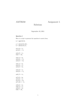
This document provides the solutions to assignment questions about linear algebra and linear programming. It includes: 1) The matrix and vector representations of a system of linear equations. It finds the numerical solution and compares it to the exact solution. 2) An analysis of the condition number of Hilbert matrices of increasing size, showing the condition number grows exponentially up to a certain point. 3) Formulating a production planning problem as a linear programming problem to maximize profit subject to resource constraints. It solves the problem as both a linear program and integer program.

1. AMTH250 Assignment 5
Solutions
September 16, 2011
Question 1
Here is a script to generate the equations in matrix form:
k = sqrt(2)/2;
a = zeros(13,13);
b = zeros(13,1);
a(1,2) = 1;
a(1,6) = -1;
a(2,3) = 1;
b(2) = 10;
a(3,1) = k;
a(3,4) = -1;
a(3,5) = -k;
a(4,1) = k;
a(4,3) = 1;
a(4,5) = k;
a(5,4) = 1;
a(5,8) = -1;
a(6,7) = 1;
a(7,5) = k;
a(7,6) = 1;
a(7,9) = -k;
a(7,10) = -1;
a(8,5) = k;
a(8,7) = 1;
a(8,9) = k;
b(8) = 15;
1

2. a(9,10) = 1;
a(9,13) = -1;
a(10,11) = 1;
b(10) = 20;
a(11,8) = 1;
a(11,9) = k;
a(11,12) = -k;
a(12,9) = k;
a(12,11) = 1;
a(12,12) = k;
a(13,13) = 1;
a(13,12) = k;
% Exact solution
x0 =[-20*sqrt(2) 20 10 -30 10*sqrt(2) 20 0 -30 5*sqrt(2) 25 20 -25*sqrt(2) 25]’;
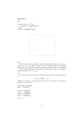
(a)
Solving in Octave:
octave:> x = ab
x =
-28.28427
20.00000
10.00000
-30.00000
14.14214
20.00000
0.00000
-30.00000
7.07107
25.00000
20.00000
-35.35534
25.00000
The accuracy can be estimated using the condition number of the matrix:
octave:> rerr =cond(a)*eps
rerr = 2.3120e-15
(b)
The actual error is
octave:> err = norm(x-x0)/norm(x0)
err = 1.3820e-16
2

3. (c)
octave:> eig(a)
ans =
-1.27279 + 0.00000i
-0.49903 + 1.07138i
-0.49903 - 1.07138i
-0.52561 + 0.56675i
-0.52561 - 0.56675i
-0.12363 + 0.93904i
-0.12363 - 0.93904i
1.14770 + 0.96283i
1.14770 - 0.96283i
0.87329 + 0.70838i
0.87329 - 0.70838i
0.72297 + 0.00000i
0.51150 + 0.00000i
The matrix a has three real eigenvalues The real eigenvalues and their cor-
responding eigenvectors are:
octave:> [V L] = eig(a);
octave:> real([L(1,1) L(12,12) L(13,13)])
ans =
-1.27279 0.72297 0.51150
octave:> real([V(:,1) V(:,12) V(:,13)])
ans =
0.2707445 -0.2173918 -0.1703240
0.1057564 0.3980937 0.3917440
-0.1346055 0.2878090 0.2003763
-0.2821253 -0.1321592 -0.0946017
0.4274406 -0.3247553 -0.1814827
0.4503570 0.5552610 0.4788643
-0.5732094 0.4014359 0.2449382
0.2619164 0.1026285 -0.0017736
-0.0882485 -0.1380302 -0.1661952
0.0854298 0.1330010 0.3427691
-0.1087340 0.0961555 0.1753257
0.0864365 -0.0912040 -0.2955285
-0.0268920 0.2327925 0.4277776
3

4. Question 2
(a)
octave:> for n = 1:30
> chilb(n) = cond(hilb(n));
> end
octave:> semilogy(chilb)
1020
15
10
1010
105
100
0 5 10 15 20 25 30
(b)
This shows that the condition number grows exponentially with n up to
about n = 12. After that it appears to to be fairly constant, but what has
happened is that rounding errors have taken over and the results are unreliable.
Note that the departure from linearity in the graph occurs at a condition
number of about 1016 ≈ 1/εmach .
(c)
An estimate for relative error in the solution of a system of linear equations
is
Erel ≈ cond Hn × εmach
Therefore to obtain a relative error less than 10−4 we require the condition
number to be less than
octave:20> 1e-4/eps
ans = 4.5036e+11
octave:> chilb(8)
ans = 1.5258e+10
octave:> chilb(9)
ans = 4.9315e+11
So n ≤ 8.
4

5. (d)
Here is a script to compute the maximum and minimum eigenvalues:
maxeig = zeros(30,1);
mineig = zeros(30,1);
for n = 1:30
eighilb = abs(eig(hilb(n)));
maxeig(n) = max(eighilb);
mineig(n) = min(eighilb);
end
0
2 10
1.8
10-5
1.6
10-10
1.4
10-15
1.2
1 10-20
0 5 10 15 20 25 30 0 5 10 15 20 25 30
Figure 1: Maximum and minimum eigenvalues of Hn (n.b. minimum eigenvalues
use semilog scale)
The maximum eigenvalue grows slowly with n increasing from 1 at n = 1 to
just less than 2 at n = 30.
The minimum eigenvale decreases exponentially with n up to about n = 12.
After that it appears to to be fairly constant, but again what has happened is
that rounding errors have taken over and the results are unreliable.
The departure from linearity in the graph occurs at a minimum eigenvalue
of about 10−16 ≈ εmach .
(e)
Experimentation shows that the computed eigenvalues are all positive up to
n = 12. For n ≥ 13 the computed eigenvalues contain some negative values.
5

6. (f )
octave:> [chilb(1:12) maxeig(1:12) mineig(1:12) maxeig(1:12)./mineig(1:12)]
ans =
1.0000e+00 1.0000e+00 1.0000e+00 1.0000e+00
1.9281e+01 1.2676e+00 6.5741e-02 1.9281e+01
5.2406e+02 1.4083e+00 2.6873e-03 5.2406e+02
1.5514e+04 1.5002e+00 9.6702e-05 1.5514e+04
4.7661e+05 1.5671e+00 3.2879e-06 4.7661e+05
1.4951e+07 1.6189e+00 1.0828e-07 1.4951e+07
4.7537e+08 1.6609e+00 3.4939e-09 4.7537e+08
1.5258e+10 1.6959e+00 1.1115e-10 1.5258e+10
4.9315e+11 1.7259e+00 3.4997e-12 4.9315e+11
1.6025e+13 1.7519e+00 1.0931e-13 1.6027e+13
5.2153e+14 1.7749e+00 3.4480e-15 5.1476e+14
1.6620e+16 1.7954e+00 1.0942e-16 1.6408e+16
λmax (Hn )
cond(Hn ) =
λmin (Hn )
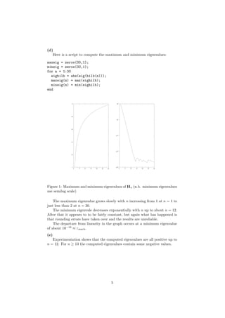
(g)
Negative eigenvalues occur for n ≥ 13. The values of the condition number
and minimum eigenvalue exhibit a change after n = 12. That these changes
occurs when the condition number reaches 1/εmach and the minimum eigenvalue
reaches εmach indicate that rounding error could well be the cause. Therefore it is
reasonable to conclude that the results for the condition number and minimum
eigenvalue are only reliable up to n = 12. There is no indication that the
computation of the maximum eigenvalue is unreliable for any of the values of n
we have looked at.
6

7. Question 3
The formulation as a linear programming problem is:
Variables: A, B, C, D, E — number of units of each product manufactured.
Objective: Maximize the profit:
c =10A + 9B + 10C + 9.5D + 5E
9
− (15A + 8B + 8C + 12D + 9E)
60
9
− (8A + 10B + 12C + 4D + 4E)
60
12
− (6A + 9B + 10C + 12D + 0E)
60
=5.35A + 4.5B + 5C + 4.7D + 3.05E
Constraints:
15A + 8B + 8C + 12D + 9E ≤ 4800
8A + 10B + 12C + 4D + 4E ≤ 4800
6A + 9B + 10C + 12D + 0E ≤ 4800
Lower Bounds:
A ≥ 0, B ≥ 0, C ≥ 20, D ≥ 30, E≥0
It is a little unclear whether this a linear programming problem or integer
programming problem; i.e. whether fractions of a product can be produced and
sold. Thefore we will solve both the LP and IP problems.
Here is the Octave script to solve both problems
obj = [5.35 4.5 5 4.7 3.05]’;
vtype1 = "CCCCC";
vtype2 = "IIIII";
ptype = -1;
cnstr=[15 8 8 12 9; 8 10 12 4 4; 6 9 10 12 0];
lb = [0 0 20 30 0]’;
ub = [];
rhs = [4800 4800 4800]’;
ctype = "UUU";
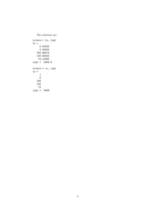
[lx, lopt] = glpk(obj, cnstr, rhs, lb, ub, ctype, vtype1, ptype);
[ix, iopt] = glpk(obj, cnstr, rhs, lb, ub, ctype, vtype2, ptype);
7

8. The solutions are:
octave:> lx, lopt
lx =
0.00000
0.00000
334.88372
120.93023
74.41860
lopt = 2469.8
octave:> ix, iopt
ix =
1
6
330
120
73
iopt = 2469
8